EVALUATION OF STRING CONSTRAINT SOLVERS USING DYNAMIC SYMBOLIC EXECUTION
by
Scott Kausler
A thesis
submitted in partial ful llment
of the requirements for the degree of
Master of Science in Computer Science
Boise State University
August 2014
c 2014
Scott Kausler
ALL RIGHTS RESERVED
BOISE STATE UNIVERSITY GRADUATE COLLEGE
DEFENSE COMMITTEE AND FINAL READING APPROVALS
of the thesis submitted by
Scott Kausler
Thesis Title: Evaluation of String Constraint Solvers Using Dynamic Symbolic Execution
Date of Final Oral Examination: 2 May 2014
The following individuals read and discussed the thesis submitted by student Scott Kausler, and they evaluated his presentation and response to questions during the final oral examination. They found that the student passed the final oral examination.
Elena Sherman, Ph.D. Chair, Supervisory Committee
Tim Andersen, Ph.D. Member, Supervisory Committee
Dianxiang Xu, Ph.D. Member, Supervisory Committee
The final reading approval of the thesis was granted by Elena Sherman, Ph.D., Chair of the Supervisory Committee. The thesis was approved for the Graduate College by John R. Pelton, Ph.D., Dean of the Graduate College.
ACKNOWLEDGMENTS
The author would rst and foremost like to express his thanks to the Computer Science faculty at Boise State University. Speci cally, the author would like to thank Dr. Elena Sherman for all of her e ort in mentoring and assisting him on his research throughout the past year. The author also appreciates the support of his other committee members, Dr. Tim Anderson and Dr. Dianxiang Xu. In addition, he would like to thank Dr. Amit Jain for his aid throughout the admission process and the authors first year of graduate school. Obviously, comparisons of string constraint solvers would be impossible without any string constraint solvers. Therefore, the author thanks the developers of the string constraint solvers used for making their solvers available and for providing additional insight into their solvers. In particular, the author recognizes Muath Alkhalaf and his fellow STRANGER developers for providing insight into the differences of string constraint solvers. Finally, the author thanks his parents for their everlasting support and his brother for encouraging him to study computer science. This research was supported with funding from the IGEM grant.
ABSTRACT
Symbolic execution is a path sensitive program analysis technique used for error detection and test case generation. Symbolic execution tools rely on constraint solvers to determine the feasibility of program paths and generate concrete inputs for feasible paths. Therefore, the e ectiveness of such tools depends on their constraint solvers. Most modern constraint solvers for primitive data types, such as integers, are both efficient and accurate. However, the research on constraint solvers for complex data types, such as strings, is ongoing and less converged. For example, there are several types of string constraint solvers provided by researchers. However, a potential user of a string constraint solver likely has no comprehensive means to identify which solver would work best for a particular problem.
In order to help the user with selecting a solver, in addition to the commonly used performance criterion, we introduce two criteria: modeling cost and accuracy. Using these selection criteria, we evaluate four string constraint solvers in the context of symbolic execution. Our results show that, depending on the needs of the user, one solver might be more appropriate than another, yet no solver exhibits the best overall results. Hence, we suggest that the preferred approach to solving constraints for complex types is to execute all solvers in parallel and enable communication between solvers.
TABLE OF CONTENTS
ABSTRACT…………………………………………
LIST OF TABLES…………………………………….
LIST OF FIGURES……………………………………
LIST OF ABBREVIATIONS …………………………….
1 Introduction……………………………………….
1.1 Symbolic Execution . . . . . . . . . . . . . . . . . . . . . . . . . . . . . . . . . . . . . . . .
1.1.1 Description . . . . . . . . . . . . . . . . . . . . . . . . . . . . . . . . . . . . . . . . .
1.1.2 Example . . . . . . . . . . . . . . . . . . . . . . . . . . . . . . . . . . . . . . . . . . .
1.2 Constraint Solvers . . . . . . . . . . . . . . . . . . . . . . . . . . . . . . . . . . . . . . . . .
1.2.1 Constraint Solvers in Symbolic Execution. . . . . . . . . . . . . . . . . .
1.3 String Constraint Solvers . . . . . . . . . . . . . . . . . . . . . . . . . . . . . . . . . . . .
1.3.1 Example . . . . . . . . . . . . . . . . . . . . . . . . . . . . . . . . . . . . . . . . . . .
1.3.2 String Constraint Solver Characteristics . . . . . . . . . . . . . . . . . . .
1.3.3 String Constraint Solver Evaluation . . . . . . . . . . . . . . . . . . . . . .
1.4 Dynamic Symbolic Execution. . . . . . . . . . . . . . . . . . . . . . . . . . . . . . . . .
1.5 Thesis Statement . . . . . . . . . . . . . . . . . . . . . . . . . . . . . . . . . . . . . . . . . .
2 Current Tools and Methods……………………………
2.1 Overview . . . . . . . . . . . . . . . . . . . . . . . . . . . . . . . . . . . . . . . . . . . . . . . .
2.2 Automata -Based Solvers. . . . . . . . . . . . . . . . . . . . . . . . . . . . . . . . . . . . .
2.2.1 Examples. . . . . . . . . . . . . . . . . . . . . . . . . . . . . . . . . . . . . . . . . . .
2.2.2 Automata Solver Clients. . . . . . . . . . . . . . . . . . . . . . . . . . . . . . .
2.3 Bit-vector Based Solvers. . . . . . . . . . . . . . . . . . . . . . . . . . . . . . . . . . . . .
2.3.1 Examples. . . . . . . . . . . . . . . . . . . . . . . . . . . . . . . . . . . . . . . . . . .
2.3.2 Bit-vector Solver Clients . . . . . . . . . . . . . . . . . . . . . . . . . . . . . . .
2.4 Other Solvers . . . . . . . . . . . . . . . . . . . . . . . . . . . . . . . . . . . . . . . . . . . . .
2.4.1 Examples. . . . . . . . . . . . . . . . . . . . . . . . . . . . . . . . . . . . . . . . . . .
2.5 Related Work on Comparison of String Constraint Solvers . . . . . . . . . .
3 Metrics for String Sovler Comparisons……………………
3.1 Example . . . . . . . . . . . . . . . . . . . . . . . . . . . . . . . . . . . . . . . . . . . . . . . . .
3.2 Performance . . . . . . . . . . . . . . . . . . . . . . . . . . . . . . . . . . . . . . . . . . . . . .
3.3 Modeling Cost . . . . . . . . . . . . . . . . . . . . . . . . . . . . . . . . . . . . . . . . . . . .
3.4 Accuracy. . . . . . . . . . . . . . . . . . . . . . . . . . . . . . . . . . . . . . . . . . . . . . . . .
3.5 Measurements of Accuracy. . . . . . . . . . . . . . . . . . . . . . . . . . . . . . . . . . .
3.5.1 Measure 1: Unsatis able Branching Points. . . . . . . . . . . . . . . . .
3.5.2 Measure 2: Singleton Branching Points. . . . . . . . . . . . . . . . . . . .
3.5.3 Measure 3: Disjoint Branching Points. . . . . . . . . . . . . . . . . . . . .
3.5.4 Measure 4: Complete Branching Points . . . . . . . . . . . . . . . . . . .
3.5.5 Measure 5: Subset Branching Points. . . . . . . . . . . . . . . . . . . . . .
3.5.6 Measure 6: Additional Value Branching Points. . . . . . . . . . . . . .
3.5.7 Measure 7:Top Operations. . . . . . . . . . . . . . . . . . . . . . . . . . . . .
3.5.8 Hierarchy of Accuracy. . . . . . . . . . . . . . . . . . . . . . . . . . . . . . . . .
3.6 Dynamically Comparing Solvers. . . . . . . . . . . . . . . . . . . . . . . . . . . . . . .
4 String Solver Analysis Framework……………………….
4.1 Overview . . . . . . . . . . . . . . . . . . . . . . . . . . . . . . . . . . . . . . . . . . . . . . . .
4.2 Instrumenter. . . . . . . . . . . . . . . . . . . . . . . . . . . . . . . . . . . . . . . . . . . . . .
4.3 Collector. . . . . . . . . . . . . . . . . . . . . . . . . . . . . . . . . . . . . . . . . . . . . . . . .
4.4 Processor . . . . . . . . . . . . . . . . . . . . . . . . . . . . . . . . . . . . . . . . . . . . . . . .
4.5 Constraint Solvers . . . . . . . . . . . . . . . . . . . . . . . . . . . . . . . . . . . . . . . . .
4.5.1 EJSA. . . . . . . . . . . . . . . . . . . . . . . . . . . . . . . . . . . . . . . . . . . . . .
4.5.2 ESTRANGER. . . . . . . . . . . . . . . . . . . . . . . . . . . . . . . . . . . . . . .
4.5.3 EZ3-str . . . . . . . . . . . . . . . . . . . . . . . . . . . . . . . . . . . . . . . . . . . .
4.5.4 EECLiPSe-str . . . . . . . . . . . . . . . . . . . . . . . . . . . . . . . . . . . . . . .
4.6 Summary . . . . . . . . . . . . . . . . . . . . . . . . . . . . . . . . . . . . . . . . . . . . . . . .
5 The Evaluator ……………………………………..
5.1 Performance . . . . . . . . . . . . . . . . . . . . . . . . . . . . . . . . . . . . . . . . . . . . . .
5.2 Modeling Cost . . . . . . . . . . . . . . . . . . . . . . . . . . . . . . . . . . . . . . . . . . . .
5.3 Measurements of Accuracy. . . . . . . . . . . . . . . . . . . . . . . . . . . . . . . . . . .
5.3.1 Measure 1: Unsatis able Branching Points. . . . . . . . . . . . . . . . .
5.3.2 Measure 2: Singlet on Branching Points. . . . . . . . . . . . . . . . . . . .
5.3.3 Measure 3: Disjoint Branching Points. . . . . . . . . . . . . . . . . . . . .
5.3.4 Measure 4: Complete Branching Points . . . . . . . . . . . . . . . . . . .
5.3.5 Measure 5: Subset Branching Points. . . . . . . . . . . . . . . . . . . . . .
5.3.6 Measure 6: Additional Value Branching Points. . . . . . . . . . . . . .
5.3.7 Measure 7: Top Operations. . . . . . . . . . . . . . . . . . . . . . . . . . . . .
5.4 Debugging . . . . . . . . . . . . . . . . . . . . . . . . . . . . . . . . . . . . . . . . . . . . . . .
5.5 Summary . . . . . . . . . . . . . . . . . . . . . . . . . . . . . . . . . . . . . . . . . . . . . . . .
6 Results…………………………………………..
6.1 Modeling Cost . . . . . . . . . . . . . . . . . . . . . . . . . . . . . . . . . . . . . . . . . . . .
6.2 Performance . . . . . . . . . . . . . . . . . . . . . . . . . . . . . . . . . . . . . . . . . . . . . .
6.3 Accuracy. . . . . . . . . . . . . . . . . . . . . . . . . . . . . . . . . . . . . . . . . . . . . . . . .
6.4 Recommendations. . . . . . . . . . . . . . . . . . . . . . . . . . . . . . . . . . . . . . . . . .
7 Conclusion and Future Work…………………………..
7.1 Comparison of String Constraint Solvers . . . . . . . . . . . . . . . . . . . . . . . .
7.2 Future Work. . . . . . . . . . . . . . . . . . . . . . . . . . . . . . . . . . . . . . . . . . . . . .
7.2.1 Comparisons . . . . . . . . . . . . . . . . . . . . . . . . . . . . . . . . . . . . . . . .
7.2.2 Constraint Solver Development. . . . . . . . . . . . . . . . . . . . . . . . . .
7.3 Final Note . . . . . . . . . . . . . . . . . . . . . . . . . . . . . . . . . . . . . . . . . . . . . . .
REFERENCES……………………………………….
LIST OF TABLES
3.1 Variations in modeling cost, accuracy, and performance. . . . . . . . . . . . .
3.2 Displays the importance of each measurement of accuracy. . . . . . . . . . .
4.1 Available interfaces used in the extended solvers.. . . . . . . . . . . . . . . . . .
4.2 Describes the methods modeled by each extended string constraint solver.
6.1 Program artifacts and constraint descriptions. . . . . . . . . . . . . . . . . . . . .
LIST OF FIGURES
1.1 An integer based code snippet that may be explore using SE. . . . . . . . .
1.2 A symbolic execution tree fort he code in Figure 1.1.. . . . . . . . . . . . . . .
1.3 Demonstrates a SQ L query generate dusing JDBC that could produce a run time error due to a missing space between a d dress and WHERE. .
2.1 Example code snippet. . . . . . . . . . . . . . . . . . . . . . . . . . . . . . . . . . . . . . .
2.2 Constraint graph for the code snippet in Figure 2.1. . . . . . . . . . . . . . . .
2.3 Automaton representing any string. . . . . . . . . . . . . . . . . . . . . . . . . . . . .
2.4 No deterministic automat on representing foo . . . . . . . . . . . . . . . . . . . .
2.5 Nondeterministic automaton representing foo concatenated with any string. . . . . . . . . . . . . . . . . . . . . . . . . . . . . . . . . . . . . . . . . . . . . . . . . . . .
3.1 A disjoint branching point.. . . . . . . . . . . . . . . . . . . . . . . . . . . . . . . . . . .
3.2 Anon-disjoint branching point. . . . . . . . . . . . . . . . . . . . . . . . . . . . . . . .
3.3 Approximation a affects satisability result. . . . . . . . . . . . . . . . . . . . . . . .
3.4 Approximation does not a affect satisability result.. . . . . . . . . . . . . . . . .
3.5 A code snippet that demonstrates a singlet on branching point and a singlet on hot spot. . . . . . . . . . . . . . . . . . . . . . . . . . . . . . . . . . . . . . . . . . .
3.6 Asubset branching point that falls under case one. . . . . . . . . . . . . . . . .
3.7 A sub set branching point that falls under case two. . . . . . . . . . . . . . . . .
4.1 Diagram of SSAF. . . . . . . . . . . . . . . . . . . . . . . . . . . . . . . . . . . . . . . . . .
4.2 Example demonstrates multiple address code. . . . . . . . . . . . . . . . . . . . .
4.3 Demonstrates three-address code.. . . . . . . . . . . . . . . . . . . . . . . . . . . . . .
4.4 Instrumented code and the corresponding CG. Based on code in Figure 2.1.58
4.5 No deterministic automata that were independently created by extracting the first two and last character of the string foo . . . . . . . . . . . . . .
4.6 No deterministic automaton representing foo after bar has been inserted at index 2. . . . . . . . . . . . . . . . . . . . . . . . . . . . . . . . . . . . . . . . . .
4.7 Nondeterministic automaton representing foo after ignore case operation. . . . . . . . . . . . . . . . . . . . . . . . . . . . . . . . . . . . . . . . . . . . . . . . . . .
5.1 An unsound branching point. . . . . . . . . . . . . . . . . . . . . . . . . . . . . . . . . .
6.1 Uses methods encountered on the x-axis to display modeling cost and characteristics of our test suite. . . . . . . . . . . . . . . . . . . . . . . . . . . . . . . .
6.2 Y-axis displays the average time per branching point in seconds. . . . . .
6.3 Y-axis displays the median time per branching point in seconds.. . . . . .
6.4 A code snippet that will not produce unsatisfiable branching points.. . .
6.5 Displays accuracy in our test suite. . . . . . . . . . . . . . . . . . . . . . . . . . . . .
LIST OF ABBREVIATIONS
API – Application Programming Interface
BDD- Binary Decision Diagram
BEA – Beasties
CG -Constraint Graph
CLP – Constraint Logic Programming
CSP – Constraint Satisfaction Problem
DFA – Deterministic Finite Automata
DSE – Dynamic Symbolic Execution
FG – Flow Graph
HCL- Html Cleaner
ITE – iText
JHP- Jericho HTML Parser
JNA- Java Native Access
JPF -Java PathFinder
JSA- Java String Analyzer
JST- Java String Testing
JXM – jxml2sql
LOC- Lines of Code
M2L- Monadic Second-Order Logic
MPJ- MathParser Java
MQG- MathQuiz Game
NCL -Natural CLI
NFA -Nondeterministic Finite Automata
OCL- Object Constraint Language
parray- Paramertized Array
PC- Path Condition
SE- Symbolic Execution
SML- String Manipulation Library
SMT- Satis ability Modulo Theory
SPC– Symbolic Path Finder
SSAF String Solver Analysis Framework
CHAPTER 1
INTRODUCTION
1.1 Symbolic Execution
1.1.1 Description
Symbolic execution (SE) [26, 10] is a path sensitive static program analysis technique that is useful for error detection, test case generation, and SQL injection attack generation. SE interprets programs using symbolic instead of concrete input values, e.g., numbers. These symbolic values are initially unrestricted, i.e., they can represent
any concrete value. Upon reaching a branching point, i.e., a conditional statement, SE follows either a true or false branch. When following the selected branch, SE generates a constraint corresponding to that branch and conjoins it with the constraints of the previously taken branches. Thus, the resulting conjunction of constraints, called the path condition or PC, is the conjunction of all constraints along the explored path. A PC represents all concrete values that variables can evaluate to at that point during concrete executions that follow the same path.
1.1.2 Example
SE is an e ective tool for describing all values that can occur at specific points in a program. In addition, it detects infeasible paths within a program. For example,
1. int x,y;
2. if (x > y) {
3. x = x + y;
4. y = x- y;
5. x = x- y;
6. if (x > y)
7. assert false;
8. }
Figure 1.1: An integer based code snippet that may be explore using SE.
consider how the code in Figure 1.1 is analyzed by SE. Figure 1.2 depicts the codes SE tree [30]. At line 1, SE assigns symbolic values X for variable x and Y for variable y. In concrete execution, i.e., when executing a program normally, X and Y are concrete values, but in SE we cannot make any assumptions about these values because we want to reason about all potential concrete values for x and y. The symbolic values are initially unrestricted and the PC is initially assigned to true. However, at line 2, two separate constraints are generated and independently extend the PC to re ect the outcome of each branch. The rst branch, represented by node 3 in Figure 1.2, assumes the branching point at line 2 is true, so the PC is conjoined with the constraint X > Y. The second branch, which leads to node 8a in Figure 1.2, assumes the branching point is false and conjoins the PC with the constraint X Y .
We now have two separate PCs that represent two di erent paths. If we continue to explore the true path for the branching point at line 2, we encounter an assignment statement at line 3 that changes the value of x. The right hand side of this statement must be expressed in terms of symbolic values X and Y , so the symbolic state is updated so that the value of variable x is X +Y . We use this value for x at line 4, where we update the symbolic state so that y = X +Y Y (or y = X). At line 5, the state is again updated so that x = X + Y X (or x = Y).
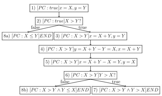
Figure 1.2: A symbolic execution tree for the code in Figure 1.1.
Notice that the symbolic values for x and y are now swapped due to the assignment statements in lines 3-5 so that x has symbolic value Y and y has symbolic value X. These updated symbolic values for x and y are used in the generation of constraints for the branching point at line 6. At line 6, the constraint Y X is added to the PC to generate the false condition. The final PC for the true branch of the first branching point and the false branch of the second branching point now states X > Y Y X. In some cases, SE might re ne this PC to a simpler form, i.e., X > Y. The true branch of the branching point at line 6 adds Y > X to the PC so that it reads: X > Y Y > X. Notice that there are no values for X and Y that could satisfy this PC because X cannot be both less than and greater than Y , which means the PC is unsatis able. It also means that the path is infeasible and there are no concrete input values that can lead to that path. In other words, the path will never be taken in concrete execution. If SE detects an unsatis able PC, it does not explore that path. In order to detect infeasible paths such as the true branch at line 6 in Figure 1.1, SE must use a constraint solver to solve the conjunction of constraints. If the constraint solver can detect an unsatis able PC, it reports this result to the SE tool. Furthermore, SE uses a constraint solver to nd values that might occur at a hotspot, which we define as follows:
Deffenition 1.1. A hotspot is a program point where an interesting value or expression is located.
An error or injection attack can be found by conjoining the PC at a hotspot with an error or injection attack pattern, and a test case can be found by generating inputs that lead to a hotspot. The ability to detect unsatis able PCs is an essential feature in SE. If a constraint solver is used to detect an error by solving a constraint, and it incorrectly reports that the constraint is satis able, then we say it has produced a false positive, which essentially means the constraint solvers result caused the SE tool to report an error that doesnt exist. For example, if we use SE to detect an error at a hotspot by conjoining constraints that represent an error pattern to a PC, then SE will always report that an error is present if its constraint solver cannot detect an unsatis able PC, regardless of if there is an actual error.
In the constraint generation phase, which is SEs first phase, SE systematically an alyzes all possible paths in a program and generates PCs for that program. However, there is one major drawback to this approach. The worst case time complexity of the path exploration is exponential with respect to the number of branching points. This limitation is called the path explosion problem. Because SE suffers from the path explosion problem, only programs with few branching points can be fully analyzed by SE. In particular, identifying all paths that traverse a loop is di cult because each iteration of a loop may generate a new path.
To make SE more efficient, bounds on the number of loop iterations to be explored are used. This limits the number of paths to be explored. The example based on Figure 1.1 shows another technique employed by SE to limit the number of paths to be explored and improve efficiency: using a constraint solver to detect and ignore infeasible paths. Neither technique affects SEs time complexity. Because SE uses constraint solvers to improve efficiency and solve PCs at hotspots, the e ectiveness of a SE tool is dependent on its constraint solvers.
1.2 Constraint Solvers
1.2.1 Constraint Solvers in Symbolic Execution
When SE makes use of a constraint solver to solve constraints, it enters its second phase, called the constraint solving phase. There are two cases that cause SE to enter the constraint solving phase. The first case is when the SE tool performs a check to determine if a PC is satisfiable when a branching point is encountered. The second
case is when the SE tool encounters a hotspot. At a hotspot, the constraint solver is often used to generate test cases, generate injection attacks, or detect errors. In either case, the SE tool sends a PC where the variables take symbolic values to the solver to determine whether or not it is satisfiable. First, the constraint solver attempts to find a solution for the PC. If the solver determines that a solution cannot be found, then it reports that the PC is unsatis able by returning UNSAT. If the solver can find a solution, then it reports that the PC is satisfiable, by returning SAT,
and produces a solution, i.e., concrete values of symbolic values, that satis es the PC. In addition, some constraint solvers may report a solution for all concrete values that are represented by a symbolic value in a PC, instead of just one. In order to generate test cases, a constraint solver returns concrete values for initial symbolic values in a satisfiable PC, e.g., 1 for X in the example given for Figure 1.1.
These concrete values can then be used to execute the program along the same path represented by the PC.
In order to detect an error or injection attack at a hotspot, invalid patterns can be encoded as a set of constraints then conjoined with a PC. Any satisfying assignment for this conjoined constraint represents a value that is both invalid and satisfies the original PC, i.e., it indicates the presence of an error or injection attack. Constraint
solvers that are capable of producing values that lead to a hotspot, i.e., concrete assignments to initial symbolic values, can also produce an invalid set of inputs.
We now present several de nitions that will be used throughout the remainder of this thesis:
Definition 1.2.
A sound constraint solver will never report that a satis able PC is un satisfiable.
Definition 1.3.
A complete constraint solver will never report that an unsatisfiable
PC is satis able.
A complete constraint solver will never report any false positives, i.e., it does not produce any solutions that cannot evaluate a PC to true.
Definition 1.4.
An accurate constraint solver is both sound and complete.
Definition 1.5.
Over-approximation occurs when a solution of a constraint is sound but incomplete. An over-approximated solution might add concrete values that cannot evaluate a PC to true but never misses a concrete value.
Definition 1.6.
Under-approximation occurs when a solution of a constraint is complete but unsound. An under-approximated solution might miss concrete values that occur given a PC but does not add extra concrete values.
As a rule, constraint solvers must be sound but may or may not be complete, meaning a constraint solver must report all values that actually occur given the constraint but may include extra values, i.e., values may be over approximated but never under-approximated. This means that a trivial (but useless) constraint solver can report that all paths are satisfiable and any value can occur at any hotspot. If a solver is unsound, it will report that a satis able PC is unsatis able, might not produce any test cases, and might report that there are no invalid patterns at a hotspot, when in reality there is one or more.
In general, determining if a given PC is satisfiable is an undecidable problem. For example, a constraint in the theory of linear integer arithmetic is decidable, but adding a multiplication symbol to its signature makes it non-linear integer arithmetic, which is undecidable [38]. Because determining the satisfiability of a PC is an undecidable problem, we may approximate PCs and allow results that are not complete. Some theories, such as linear integer arithmetic, are well developed, and therefore solvers like Z3 [11] solve their problems accurately and efficiently. In particular, integer arithmetic is well understood because integers have been studied by mathematicians for centuries. Other theories, such as string theory, are relatively new. For example, string theory has only existed with the advent of object oriented programming. Since each programming language has its own representation and library of strings, there are several different approaches taken towards solving string constraints, so we focus on string constraint solvers from this point on.
1.3 String Constraint Solvers
In this thesis, we apply string constraint solvers to string constraints gathered from Java programs. This means that we analyzed variables and methods that come from the java.lang.String, java.lang.StringBuilder, and java . lang . String Buffer classes. These classes describe our string types. For brevity, we may respectively refer to these classes as String, String Builder, or String Buffer. When referring to methods in these classes, we use the name and parameter type to denote a speci c method, i.e., substring(int). In addition, we use only the name when referring to all methods that share that name, e.g., substring refers to substring(int) and substring(int,int). We do not refer to the calling classes or return values of these methods because we do not need to distinguish methods using classes or return values. There are several methods present in multiple string classes, e.g., append appears in both String Builder and String Buffer, but in these cases the same approach is taken regardless of the class.
String theory is not well de ned because every programming language contains a unique library of predicates, such as contains(String), and operations, such as trim(), that may be applied to strings. Although any program that uses strings may benefit from a SE tool with a string constraint solver, web applications in particular have created a demand for string constraint solving. For example, SQL injection attacks can be prevented for an arbitrary web application if the application is analyzed using SE and the hotspots are SQL query execution points. However, identifying injection attacks requires complete solutions of string values within a string constraint solver because incomplete solutions produce false positives. Few false positives are tolerable, but no software tester will test an infinite number of false positives. An example of the importance of complete string constraint solvers is
demonstrated below.
1.3.1 Example
1. public void printAddresses(int id) throws SQLException {
2. Connection con = DriverManager.getConnection(“students.db”);
3. String q = “SELECT * FROM address”;
4. if(id!=0)
5. q = q + “WHERE studentid=” + id;
6. ResultSet rs = con.createStatement().executeQuery(q);
7. while(rs.next()){
8. System.out.println(rs.getString(“addr”));
9 }
10 }
Figure 1.3: Demonstrates a SQL query generated using JDBC that could produce a runtime error due to a missing space between address and WHERE.
Consider the code presented in Figure 1.3, which was initially featured as an example in [9]. This code uses JDBC to print addresses stored in a database of students. Line 2 creates the database connection to students.db , line 3 starts an SQL query using the String class, line 5 appends the query with a WHERE clause if the conditional statement at line 4 evaluates to true, line 6 executes the query, and lines 7-9 print the addr column of the querys result. The Java syntax is valid and will not cause a compilation error. All queries generated in the code contain the substring SELECT * FROM address . However, not all queries include the WHERE clause at line 5 due to the conditional at line 4, which means program tests may not cover queries containing this clause.
Appending the WHERE clause to the query results in a error. Queries containing the WHERE clause read as: SELECT * FROM addressWHERE studentid= + id, where id != 0 Notice that there is no space between address and WHERE . Without this space, the query is not valid SQL syntax and causes a runtime exception when the
statement is executed at line 6. Now, imagine this code gets interpreted by a SE tool. Assume a hotspot is created whenever the execute Query method is called. If there is a case where print Addresses is called with id != 0, the symbolic value generated at the hotspot in line 6 will contain the value SELECT * FROM addressWHERE studentid= + id. Given standard regular language operations where represents negation, represents concatenation, represents the empty string, represents Kleene closure, represents disjunction, [a b] represents any numeral between a and b (inclusive), and concrete strings are surrounded by , assume the regular expression constraint ( SELECT * FROM address ( WHERE studentid= (- ) [1 9] [0 9] )) is conjoined with the PC for the hotspot at line 6. Because the regular expression matches strings that are NOT of the form SELECT * FROM address or SELECT * FROM address WHERE studentid= + id, the resulting symbolic value will still contain SELECT * FROM addressWHERE studentid= + id. The SE tool should report that the error pattern is satisfiable, which will alert the user that a potential error has occurred. Ideally, the user will run a concrete execution of the program with values that will cause this error and verify that it exists. However, if the constraint solver is complete but unsound, the SE tool may miss the error. Furthermore, if the constraint solver is incomplete but sound, it may report several potential error values that do not cause errors. For example, it may report an error when id = 0. If the tester tests this case instead of the case where id != 0, he or she may falsely conclude that there is no error at that point.
1.3.2 String Constraint Solver Characteristics
SE tools work on different abstraction levels when modeling string constraints. Some precisely model string constraints by representing a string as an array of characters and exploring string library functions as a set of primitive functions. This approach can be ine cient, so other tools use string constraint solvers that work in a particular fragment of the theory of strings.
For example, a basic string constraint solver may only support concatenation and containment [18], while a more advanced string constraint solver might support concatenation, containment, replace, substring, and length [47, 50]. These more advanced string constraint solvers can model many predicates and operations in the String, String Builder, and StringBuffer classes, although the accuracy of the model depends on the accuracy of the basic predicates or operations. For example, an ends With predicate can usually be modeled accurately using concatenation and containment. String constraint solvers also commonly support constraints in the form of regular expressions [9, 24], which are useful for describing error patterns, describing injection attack patterns, or modeling predicates and operations. In addition to supported fragments, string constraint solvers often vary in their underlying representation of symbolic strings. These underlying representstions are usually either based on automata [9] or bit-vectors [24]. For the first representation, an unrestricted symbolic value is modeled using an automaton that accepts any string, a predicate is modeled by attempting to partition the language of an automaton, and an operation is modeled as a modification to an automaton.
Automata-based string constraint solvers are e cient because the time complexity of modifying an automaton is usually polynomial in the number of states and/or transitions in the automaton. On the other hand, bit-vector string constraint solvers work by imposing a length bound on the characters in a symbolic value, encoding predicates and operations in some underlying formalism, such as satis ability modulo theory (SMT) or constraint satisfaction problems (CSP), searching for a solution, and increasing the length bound if no solution is found until a maximum length k is reached. If at that point no solutions can be found, the result is unsatis able. This length requirement allows bit vector string constraint solvers to naturally keep track of the length of the underlying string, whereas automata-based string constraint solvers must use other techniques to keep track of a strings length.
Unfortunately, this length requirement also causes bit-vector solvers to be inecient. In order to support multiple variables, which is a requirement in a constraint solver for SE, bit-vector solvers must iterate over every combination of lengths. Usually, this iteration requires more time than SE will allow, so bit-vector solvers must take an alternate approach to be used in SE. Such alternate approaches often involve solving any constraints on length before encoding a string as a bounded bit-vector [6]. A constraint solver may or may not incrementally solve constraints in a PC. An incremental constraint solver can store a previous conjunction of constraints in an intermediate form. This intermediate form allows the user to add one constraint at a time to a PC while still collecting the result of the entire PC. This is advantageous for reusing the pre x of a PC. A PC pre x is de ned as follows:
Definition 1.7.
A PC pre x is the conjunction of constraints in the beginning of a PC. For example, a PC composed of constraints c1 ck might have a pre x c1 ci, where 1 i < k.
Incrementally solving constraints saves time when solving PCs that contain the same pre x. Because SE attempts to explore every path in the program, it often reuses pre xes, so it bene ts from using an incremental constraint solver. An automaton may serve as an intermediate form, so automata-based string constraint solvers are naturally incremental.
1.3.3 String Constraint Solver Evaluation
Despite the underlying di erences, all string constraint solvers may be evaluated using the same metrics. These metrics fall under the categories of performance, modeling cost, and accuracy.
Performance can be measured by keeping track of the time required for evaluation of several PCs. However, complications arise when comparing incremental and non incremental constraint solvers. In order to compare performance of both types of solvers, for incremental solvers we incrementally keep track of the time required to evaluate the whole PC, instead of only measuring the time required to add a constraint to the PC. In order to make our analysis diverse, we measure PCs taken from long program paths. Modeling cost is based on the e ort required to use a constraint solver. This is a useful metric for comparison because users want to spend as little time as possible understanding and extending a constraint solver for use in their analyses. It is difficult to conclusively measure accuracy for a string constraint solver. Instead, there are several different metrics that help indicate accuracy. When measuring accuracy, we include rudimentary checks to ensure the constraint solvers are at least partially sound. However, in general, we assume the solvers are sound.
Therefore, our measures of accuracy deal with observing over-approximation. There are two causes of over-approximation. The first cause is from an incomplete model of an operation. It is hard to tell which operations are over-approximated by a string constraint solver, so we must assume over-approximation is introduced in all
future constraints that involve a modified symbolic value. The second cause of over-approximation comes from predicates at branching points. Fortunetely, we know that if complementary predicates for a branching point create two disjoint sets from the values represented by a symbolic value, then the branching point has not be over-approximated. Therefore, when the constraints generated by two branches of a branching point do not create disjoint sets of values, we must assume over-approximation has been generated from the predicate for at least one branch. In addition, we must assume this over-approximation is propagated to future constraints that use the symbolic values represented by the two branches.
Although SE can be used to compare string constraint solvers, it is not the most optimal technique when using real world programs for comparison because of its tendency to only use simple PCs representing short program paths. In addition, there is no means of gathering concrete values in SE, which help in determining if a solver is accurate. Instead, we prefer to use a technique that generates PCs based on concrete execution, called dynamic symbolic execution, which we introduce in the next section.
1.4 Dynamic Symbolic Execution
Dynamic symbolic execution (DSE) [36, 12] is similar to SE, but it only generates PCs along one path in a programs execution. This path is the one taken by a concrete
execution of the program. DSE treats all input values as symbolic, even though concrete execution consists of concrete inputs. DSE collects constraints as the program follows its execution path, which requires instrumentation of the program [20]. Program instrumentation is a technique that inserts additional statements into a program to collect certain attributes. In this case, the attributes are the constraints encountered in the programs execution. Because DSE follows the programs actual execution, there is no need to check if a branch is feasible during concrete execution with DSE, since a branch must be feasible to execute it in concrete execution. In addition, DSE allows us to compare symbolic values to the actual values of variables at a given program point. Moreover, because DSE only follows one concrete path, it can analyze nontrivial PCs generated by following long paths in a programs execution. This makes it more scalable than SE. The combination of these advantages allow DSE to essentially be used to test values generated by a constraint solver, which leads us to the thesis statement.
1.5 Thesis Statement
For this thesis, the following three criteria, which we describe in Chapters 3 and 5, will be used to compare the extended string constraints solvers in Chapter 4, which are based on solvers presented in Chapter 2, and our results will be presented in Chapter 6:
. Performance: How does a solvers average time for solving PCs compare to the average time of other solvers? Is there variation between solvers in the time required to solve PCs?
. Modeling Cost: Which solver requires the least e ort to model string methods? Why might one solver require more e ort than another?
. Accuracy/over-approximation: How often are values over-approximated? When can we trust results to be accurate? In what cases do the solvers accuracies differ? Does a lack of a model for a method a affect overall accuracy?
CHAPTER 2
CURRENT TOOLS AND METHODS
2.1 Overview
This chapter rst describes works related to string constraint solvers, along with analyses that the solvers are used in. Next, it presents works in comparisons of string constraint solvers. The analyses detailed in this chapter often use a constraint graph (CG) to describe PCs, which we defined below:
Definition 2.1.
A constraint graph is a directed graph where all source vertices represent either symbolic or concrete values and all remaining vertices represent either operations or predicates encountered during execution. An edge represents the ow of data from one vertex to another.
To illustrate encoding PCs into a CG, consider how SE analyzes the code snippet in Figure 2.1. When interpreting method m(String s1, String s2), SE assigns symbolic values S1 and S2 to the rst and the second arguments of the method, respectively. When encountering the assignment statement with the substring operation, SE updates the symbolic state of the s1 variable to S1 substring(2), which means that the new symbolic value for s1 contains all substrings of the original symbolic value S1 that start at index 2. After that, an equality comparison is made
m(String s1,String s2){
s1 = s1.substring(2);
if (s1.equals(s2)) {
…
Figure 2.1: Example code snippet.
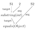
Figure 2.2: Constraint graph for the code
snippet in Figure 2.1.
between s1 and s2, and the symbolic state of each variable is updated to re affect the result.
Figure 2.2 presents a CG for the code in Figure 2.1. In this gure, the vertices labeled S1 and S2 represent initial symbolic values for variables s1 and s2. In addition, the 2 vertex represents a concrete integer value, since that value is the same in every program execution. The edges in this gure represent the ow of data from one vertex to another, i.e., they indicate that the value from one vertex is used in another vertex. The target and arg edge labels respectively denote the calling symbolic string and the argument for each method. Finally, the substring(int) and equals(Object) vertices represent string methods (substring(int) denotes an operation and equals(Object) denotes a predicate). Notice that the CG captures the value returned by the substring(int) operation with a target edge leading to the equals(Object) predicate, and S2 is the argument for equals(Object).
The CG in Figure 2.2 represents only one CG for a particular program execution. In fact, different analyses use different CGs, depending on the data they want to capture. In this way, a CG is only an abstraction of the program used to represent the data required to achieve the goals of the analysis.
Many of the analyses presented below also use a taint analysis [35], which observes data dependencies that are a ected by a prede ned source such as user input. A computation that depends on data obtained from a taint source is tainted. Other values are considered to be untainted. A taint policy determines how taint ows through a program execution.
Just like the CG depends on the type of analysis, the result of a taint analysis depends on the taint policy. For example, most taint analyses will consider s1 and s2 to be initially tainted in Figure 2.1, since they represent unknown input. Furthermore, some taint policies will consider s1 to be tainted after the substring(int) operation because it is dependent on s1s initial value. On the other hand, some policies might consider values to be untainted after the operation because it could remove potentially harmful values that might occur for s1.
If we use a conservative taint policy, then all vertices in our CG from Figure 2.2, except for 2, get tainted. Because it does not depend on user input, 2 should not be tainted. Under this conservative policy, s1 propagates taint to the substring(int) and equals(Object) vertices while s2 propagates taint to the equals(Object) vertex. String constraint solvers use various underlying representations of symbolic strings. We therefore present our survey of the solvers based on their underlying representations. These solvers are often used in SE, static analysis, dynamic analysis, and model driven analysis. Before reviewing the solvers, we must rst introduce what the terms static analysis, dynamic analysis, and model driven analysis mean. A static analysis is an analysis that interprets a program. As we mentioned in Section 1.1, SE is a static analysis technique. However, SE is a path sensitive technique, so the community often uses the term static analysis to describe path insensitive static analysis. In this type of static analysis, an abstract value describes all concrete values that might occur for a variable at a program point, instead of just the concrete values occurring along one program path.
Because static analysis might over-approximate the values of variables, it is often used in web security analyses. For example, static analysis on strings is used to detect SQL injection attacks, since this type of attack is prevalent across the Web and often times does not depend on non-string types.
On the other hand, dynamic analysis is an analysis performed on an executing program. Dynamic analysis is often used to circumvent the limitations of static analysis. Namely, it is less resource intensive, capable of analyzing deep program paths, and allows comparisons of values taken from real world programs. Instead of analyzing programs, model driven analysis analyzes models of programs. For example, it might be used to generate test cases using a program model created with a modeling language. Interest in model driven analysis was sparked by the
popularity of other analysis techniques.
The remainder of this chapter is structured as follows. First, we introduce the string constraint solvers that use each representation of symbolic strings, i.e., we introduce each type of string constraint solver. After introducing a type of solver, we provide a survey of analyses that the type of solver is used in. Finally, we present related work on comparison of string constraint solvers.
2.2 Automata-Based Solvers
An automata-based string constraint solver uses automata to represent symbolic and concrete string values. For example, an unrestricted symbolic value can be represented with the automaton shown in Figure 2.3. A nondeterministic automaton representing the concrete string foo is shown in Figure 2.4. Often times, the automata used in string constraint solvers allow operations that
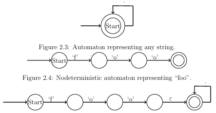
Figure 2.5: Nondeterministic automaton representing foo concatenated with any string.
are not defined for traditional automata theory. These operations manipulate the states and transitions in an automaton to model the set of strings that occur after a string method is used. For example, several automata-based string constraint solvers support substring operations. All automata-based string constraint solvers support
concatenation, so we use the automata from Figures 2.3 and 2.4 to demonstrate this operation. Typically, we implement a concatenation operation, e.g., S1 concat(S2), using automata S1 and S2 by rst creating an epsilon transition from all of S1s accept states to S2s start state then changing all of S1s accept states to non-accept states. If the automaton from Figure 2.4 represents S1 and the automaton from Figure 2.3 represents S2 in our example, the result is shown is Figure 2.5. After an operation such as this one, the automaton is then generally converted into a deterministic form. We proceed to introduce examples of automata-based string constraint solvers.
2.2.1 Examples
Christensen et al. [9] use multi-level nite automata to represent strings. Using multi-level nite automata, a minimal deterministic automaton that describes all possible values of a string variable at that program location can be extracted for every hotspot. The resulting library of automata operations is referred to as Java String Analyzer (JSA). JSAs automata are pointer based and use ranges of character values to represent transitions.
Haderach is a prototype created by Shannon et al. [37] that uses JSA as the underlying automata library, but with one major modi cation. In order to more accurately express its predicates and operations, it maintains dependencies among automata. This approach increases accuracy because changes that occur late in a PC can be applied to previous automata. Redelinghuys et al. [33] also extend JSA in their analysis. Their extension accepts a set of constraints and returns a SAT/UNSAT result along with string values, since JSA was not designed to do this. They also enhance JSA with their own routines, but do not describe what enhancements were made.
Ghosh et al. [14] present Java String Testing (JST), which analyzes hybrid string constraints by extending JSA. An example of a hybrid constraint is CharAt, which requires a comparison to a character to make any assertion. The authors required a tool with precise models of operations, so they reimplemented several of JSAs operations, such as substring, to produce a more precise result. The length is asserted in each of JSTs automata. In addition, a relaxed solving technique is used to generate satis ability results e ciently. This relaxed solving technique is not as precise, but branches after a misidenti ed unsatis able result are often found to be
unsatis able. Non-linear numeric constraints are handled by a randomized solver or a regular linear solver after being converted to a linear form.
Yu et al. [47, 48, 45, 46] present STRANGER, which uses its string manipulation library (SML) to handle string and automata operations, such as replacement, concatenation, prefix, suffix, intersection, union, and widen1. The SML,
which we refer to as STRANGER for brevity, uses the MONA library [3] to represent deterministic nite automata (DFA). In MONA, transitions are represented using Binary Decision Diagrams (BDDs).
In order to more precisely model predicates such as the not equals predicate, Yu et al. [49] introduce multi-track automata for solving string constraints. In a multi-track automaton, each track corresponds to one string value. Although this approach is empirically shown to be more precise than a standard automata approach,
it is also more resource intensive. Hooimeijer and Weimer [18] create an automata-based decision procedure for subset and concatenation constraints, as well as a prototype called DPRLE. This is the only constraint solver based on automata with proven correctness of its algorithms. Tateishi et al. [40] create an analysis that uses a BDD-based automata representation of Monadic Second-Order Logic (M2L) formulae. This implementation uses
MONAastheunderlying library. The advantage of this approach is that it can create conservative, i.e., over-approximated, models of operations and is powerful enough to model methods such as Javas replace methods.
1The SML is now open source and available at https://github.com/vlab-cs-ucsb/Stranger.
The automated validation and sanitation tool that originated as STRANGER is available at
https://github.com/vlab-cs-ucsb/SemRep.
2.2.2 Automata Solver Clients
Symbolic Execution
Shannon et al. [37] integrate symbolic strings into a SE prototype named Haderach. Traditionally in SE, the PC is stored explicitly as a list of constraints. However, Haderach represents string constraints by manipulating nite-state automata. A symbolic values automaton therefore accepts all strings that satisfy the PC for the associated variable. Haderach extends the code base of Juzi [23], which is a prototype designed to repair structurally complex data that comes from complicated structures, such as red-black trees.
Symbolic PathFinder (SPF) [31, 32] is a SE framework built on top of Java PathFinder (JPF), which is an environment for verifying Java byte code. JPF interprets byte code in a custom Virtual Machine with slot attributes that are used to store symbolic values and expressions associated with each of the locals, fields, and operands on the stack. For each path, a condition is associated with a generated choice. If the condition is unsatis able, SPF backtracks. A limit is also imposed on the depth of the search. If an expression contains a symbolic and a concrete value, the result is symbolic. Due to certain limitations, SPF is more e ective at analyzing methods than entire programs. In order to perform SE on a method, programs are executed with concrete values until a symbolic method should be analyzed. At that point, a symbolic value is injected into each variable. Alternatively, symbolic values
can be approximated based on values collected from running the program multiple times using a learning algorithm. Redelinghuys et al. [33] combine SPF with both an automata-based and a bit-vector based string constraint solver, but we do not reintroduce SPF for use with bit-vector solvers in Section 2.3.2.
Static Analysis
Christensen et al. [9] present a static program analysis technique to demonstrate the applicability of approximating the values of Java string expressions. Their analysis builds a CG to capture the ow of strings and string operations. This CG consists of Init nodes to represent new string values, Join nodes to capture assignments (or
other join points), Concat nodes to represent string concatenation, and both UnaryOp and BinaryOp nodes to represent other string operations. After building their CG, the authors construct a context-free grammar, approximate it as a regular grammar, and extract automata from this regular grammar.
STRANGER [47, 48, 45, 46] is an automata-based string analysis tool that can prove an application is free from speci ed attacks or generate a pattern characterizing malicious inputs. STRANGER uses Pixy [22] to parse a PHP program and construct a dependency graph of string operations and values with a taint analyzer. Cyclic dependencies in the graph are replaced with strongly connected components. A vulnerability analysis is conducted on the now acyclic dependency graph. In this graph, nodes are processed in a topological order using automata operations. These nodes could represent null, assign, concat, replace, restrict, and input operations. Both a forward and a backward analysis may be performed using STRANGER. Halfond and Orso [16] statically build a model of legitimate queries generated by an application. In the rst step, hotspots are identi ed. After that, SQL-query models are statically built. This is done using nondeterministic nite automata (NFA) to perform a depth rst traversal of each hotspots NFA. The depth first traversal groups characters into SQL and string tokens to obtain the SQL-query model. Then, at each hotspot the application makes a call to the runtime monitor. The runtime monitor checks dynamically generated queries against the model and rejects queries that violate the model. This is done by parsing the actual string into SQL string tokens then checking if the models automaton accepts it.
Tateishi et al. [40] perform a static analysis that is not based on a CG. Instead, the analysis encodes string assignments as operations in M2L. After the encoding, a solver is applied to check for satisfiability.
An automated static analysis technique for nding SQL injection attacks in PHP is presented by Wassermann and Su [43]. This analysis combines static taint analysis with string analysis. In order to identify substrings that may have been tainted by user input, a CG is used to maintain the relation between variables. This analyses uses Minamide [28] to model string operations.
Dynamic Analysis
Kiezun et al. [25] create a tool called Ardilla. Ardilla dynamically creates inputs that expose SQL injection and cross site scripting attacks for PHP. It executes the program with arbitrary inputs, generates constraints based on the path followed, negates a previously observed constraint, and solves the new set of constraints to mutate inputs. A taint propagator is then used to detect potential user inputs. Taint may be removed using sanitizers. Finally, candidate attack patterns are generated and verified.
In their work, Wassermann et al. [44] describe an algorithm that uses both random concrete and symbolic inputs to generate test cases for database applications based on concrete execution. The algorithm starts by executing the program on random inputs with an initial database state. It simultaneously keeps track of a path constraint and a database constraint. The algorithm looks for un executed branches in the program and adjusts future inputs to cover those branches by taking the rst unexecuted path on the next execution. Strings, records, and database relations are immutable and manipulated using an abstract data type that allows creation, comparison, and concatenation of strings. All statements are classified as either a halt, input, assignment, conditional, database manipulation, or abort statement. The constraints gathered from DSE are used to create satisfying assignments and update both the input map and database. This ensures the program gets tested while the database is in several different states.
2.3 Bit-vector Based Solvers
Bit-vector solvers encode string constraints in terms of some underlying logic, e.g., SMT, but the translation requires a bounded length on strings. This length bound allows string operations that would otherwise be undecidable but is a limitation for these solvers since they ignore solutions outside of their length bound. However, useful analyses can still be performed with these solvers, particularly if the length bound is large. Furthermore, this restriction on string length has motivated the development of solvers that do not su er from this limitation, as we discuss in Section 2.4. The solvers detailed below vary based on the logic and underlying representation of symbolic strings. However, each of the solvers below encodes each string as a vector.
2.3.1 Examples
Bj rner et al. [5] generate nite models of string path constraints using Pex. This implementation handles string functions such as concat and substring using primitives Shift and Fuse. First, the axioms for the constraints are tested for satis ability. If they are satis able, Pex then extracts values, unfolds quanti ers, and attempts to find solutions up to a bounded length.
HAMPI [24] is a bit-vector solver capable of expressing constraints in regular languages and xed size context free languages. It works by normalizing constraints into a core form, encoding them into bit-vector logic, and using the STP [13] solver to solve the bit-vector constraints. HAMPI originally only supported concatenation on single symbolic variables along with its regular and context free constraints, but the current version also supports substring operations and multiple xed length symbolic variables. HAMPI works in an NP-complete logic for its core string constraints.
Redelinghuys et al. [33] build a bit-vector based string constraint solver that uses Z3. Their implementation uses Z3s array support to solve for multiple string lengths simultaneously.
Kaluza [34] works in three steps. First, it translates string concatenation constraints into a layout of variables. Second, it extracts integer constraints on the lengths of strings to nd a satisfying length assignment. Finally, Kaluza translates the string constraints into bit-vector constraints to check for satis ability. The bit-vector constraints are solved by repeatedly invoking HAMPI.
Ulher and Dave [41] reimplement HAMPI as SHAMPI. This is done in order to demonstrate the utility of the Smten tool, which automatically translates high-level symbolic computation into SMT queries. Buttner and Cabot [6, 7] use constraint logic programming (CLP) to model string constraints. In CLP, programming is limited to the generation and solution of requirements. The solver encodes strings as bounded arrays of numbers that support length, concatenation, indexed substring, containment, and equality operations. There are three cases where the solver solves constraints.
In the first case, every valid length assignment yields a solution. In the second case, the solver can detect an unsatis ability based purely on length constraints. In the nal case, the solver generally performs poorly because elements have to be incrementally assigned values before being checked for satisfiability. Since the aforementioned solver is
unnamed, we refer to it as ECLiPSe-str from this point on.
Li and Ghosh [27] use a new structure, called a paramertized array (parray), to represent a symbolic string in their solver, called PASS. Parrays map symbolic indices to symbolic characters and use symbolic lengths. Constraints are encoded as quanti ed expressions. In addition, quanti er elimination is used to convert universally quanti ed constraints into a form that can easily be processed by SMT solvers. The algorithm used to solve these expressions is guaranteed to terminate because its search space is bounded by length. The advantage of this approach is that it can be used to detect unsatis able constraints quickly. Use of automata was avoided because they tend to over-approximate values, have weak length connections, do not extract relations between values, and must enumerate values. However, automata are still required to encode regular expressions. Automata are also used to determine unsatis ability quickly, i.e., in cases where parrays perform poorly. These automata can be converted into parrrays as needed.
2.3.2 Bit-vector Solver Clients
Symbolic Execution
Saxena et al. use dynamic symbolic execution to explore the execution space of JavaScript code in [34]. The resulting framework, called Kudzu, first investigates the event space of user interactions using a GUI explorer. After that, the dynamic symbolic interpreter records a concrete execution of the program with concrete inputs. Kudzu tracks each branching point, modifies one of the branching points, and uses a constraint solver to nd inputs that lead to the new path, so that it can cover a programs input value space. It then intersects symbolic values with attack patterns at hotspots in order to detect potential vulnerabilities.
Model Driven Analysis
In order to ensure model correctness in generating test cases based on model-driven engineering, Gonzalez et al. present EMFtoCSP2 in [15]. EMPtoCSP is based on CLP. User inputs include the model, the set of constraints over the model, and the properties to be checked. EMF3 and Object Constraint Language (OCL)4 parsers are used to translate this input. After translation, the code is sent to the ECLiPSe5 constraint programming framework to check if the model holds with the given properties. A visual display of a valid instance is then given. This display can be used as input to a program to be tested.
2.4 Other Solvers
As previously mentioned, this class of solver was developed to circumvent the limitations of bit-vector solvers. Because the length is not bounded, a more general theory must be used to impose string constraints.
2http://code.google.com/a/eclipselabs.org/p/emftocsp
3http://www.eclipse.org/modeling/emf
4http://www.eclipse.org/modeling/mdt/?project=ocl
5http://eclipseclp.org/ NOT the Eclipse IDE
2.4.1 Examples
Z3-str [50] treats strings as a primitive type within Z3. It uses Z3s theory of uninterpreted functions and equivalence classes to determine satis ability. Z3-str systematically breaks down constants and variables to denote sub-structures until the breakdown bounds the variables with constant strings or characters. When concat is detected by the Z3 core, the abstract syntax tree is passed to Z3-str using a call back function. Z3-str then applies the concat rule, reduces the tree, and sends it back to Z3s core. The split function adds a rule as the disjunction of all possible split strings. To solve, Z3-str either nds a concrete string in an equivalence class or simpli es formulas and assigns values to free variables. Substring is represented by breaking the argument into three pieces, asserting the middle piece is the return string, and asserting the proper lengths for the other pieces. Contains checks if one string is a substring of another. When contains is negated, solutions are generated for the free variables and post processing is used to check if one symbolic string is contained within the other.
2.5 Related Work on Comparison of String Constraint Solvers
The work on comparison of di erent solvers is limited, and evaluation is mainly focused on performance. For example, Hooimeijer and Weimer [19] compare their unnamed string constraint solver to DPRLE and HAMPI on a set of regular expressions and limited operations on string sets and base their comparison on performance. The unnamed solver generally exhibits the best performance in these test cases.
Hooimeijer and Veanes [17] also evaluate the performance of di erent automata based constraint solvers on basic automata operations. The authors conclude that a BDD-based representation works well when paired with lazy intersection and difference algorithms. Chapter 6 of this thesis gives another picture of performance
comparisons between automata encodings. Redelinghuys et al. [33] compare the performance of their custom implementations of bit-vector constraint solvers and their custom extension of JSA in the context of SPF.
The result is that different types of solvers perform better in separate situations, and the authors conclude that the choice of decision procedure is not important. Zheng et al. [50] compare Z3-str with Kaluza. The comparison is done both in terms of performance and correctness, although the authors do not de ne the latter. Z3-str outperforms Kaluza in 13 out of 14 test cases. Choi et al. [8] make a comparison of their approach with JSA based on performance and precision. In this case, the authors use the generality of regular expressions to determine which solver is more precise. In all cases, their approach is at least as precise as JSA. In addition, their approach is more e cient than JSA in all but one test case.
Finally, Li and Ghosh [27] compare PASS with an automata approach and an approach similar to a bit-vector one on several hundred non-trivial PCs using performance as a means of comparison. In most cases, PASS outperforms the other two approaches.
CHAPTER 3
METRICS FOR STRING SOVLER COMPARISONS
As we previously discussed, the majority the comparisons between constraint solvers are based on performance. This metric is important from the perspective of constraint solver developers, since solver competitions [39] mainly focus on performance. Even though performance is important for users, other metrics can also play critical roles in an e ective constraint solver. We speculate that at least two additional metrics, modeling cost and accuracy, should be considered when selecting an adequate solver. In this chapter, we explain in detail what they are and why they are important. In order to perform comparisons, we investigated several string constraint solvers from Chapter 2 and selected those that can be extended to model several methods in Java s String, StringBuffer and StringBuilder classes for use in our empirical evaluations. Other requirements for the solvers were the ability to handle symbolic values of variable length, e ciency, public availability, and algorithmic diversity. The following four string constraint solvers satis ed our criteria: JSA, STRANGER, Z3 str, and ECLiPSe-str. We extended each of these solvers and respectively named our extensions EJSA, ESTRANGER, EZ3-str, and EECLiPSe-str. When appropriate, we refer collectively to EJSA and ESTRANGER as the automata solvers. Since we are impartial to any of the string solvers, we used our best e ort to extend them, for example, by communicating with the developers of each solver.
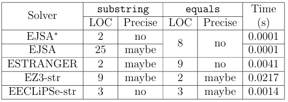
Table 3.1: Variations in modeling cost, accuracy, and performance.
3.1 Example
In order to demonstrate the importance of all three metrics in string solver com parisons, we illustrate the type of string constraints that SE can generate using the code snippet in Figure 2.1. Recall that in SE the input values for variables s1 and s2 of method m(String s1, String s2) are symbolic values S1 and S2. After the substring operation, s1s symbolic value gets updated to re ect the substring operation. To explore the true branch of the conditional statement, SE generates the following constraint:
(S1 substring(2)) equals(S2) (3.1)
This constraint restricts the concrete values of s1 to those whose substrings starting at index 2 are the same as the concrete values of s2. To determine whether it is possible to assign values S1 and S2 that can satisfy such relation between s1 and s2, i.e., whether the true branch is feasible, SE passes the above constraint to a string constraint solver. To demonstrate diversity in modeling cost, accuracy, and performance of the four string solvers, consider Table 3.1, which shows how each of the extended solvers evaluates in performance, modeling cost, and accuracy for the constraint in Formula 3.1. The rst column labels the extended string constraint solvers. Column
two displays the modeling cost in terms of number of lines of code (LOC) used to extend the substring(int) method for each extension, while column three describes accuracy by telling whether the extension might be precise or not. Columns four and five provide a similar description for the equals(Object) method. The last column shows performance as the average time in seconds that the extended string solvers require to process the two methods after ten queries. We represent accuracy in terms of the precision of method implementation, which we label as maybe or no . For equals(Object), we consider the precision of models in both the predicate and its negation. If we are certain that the model is imprecise then we label it with no . Otherwise, we label it with maybe because we lack the formal proofs required to conclusively state that the models are precise.
In this example, we have two versions of JSA extensions for the substring(int) method. The rst, EJSA, uses the built-in method, which only requires a couple of LOC to invoke. JSAs native modeling of this method over-approximates the result by allowing the resulting automaton to represent any length post x of the original automaton, not just a single substring. For example, if the symbolic string S1 from the example based on Figure 2.1 was constrained to represent the concrete string foo , the symbolic string after the native modeling of substring(2) would represent concrete strings foo , oo , o , and . In order to improve accuracy, we reimplemented the substring methods in EJSA
using the algorithm developed for JST [14]. The reimplemented substring(int,int) model advances the automaton to the starting index, sets all states reachable within the substrings length to accepts states, and restricts the new automatons length to be the length of the substring, whereas the reimplemented substring(int) model advances the automaton to the starting index. Since we cannot obtain the proof of correctness for this algorithm, we mark it as maybe accurate. Note that implementing a more precise model of the substring methods required a substantial amount of e ort. This e ort includes the labor of writing code in addition to other efforts, such as understanding the theory of automata.
Unlike JSA, STRANGER already provides a model of substring with no obvious approximations. Therefore, to achieve the same level of accuracy, we used significantly less e ort to model this string operation. However, neither of our automata-based solvers could model the equals method without introducing over-approximation. This is because automata-based solvers cannot easily capture the complex interaction between symbolic values in the false conditions of predicates such as this one and are forced to over-approximate to remain sound. We provide an explanation of this over-approximation in Section 4.5.1.
For EZ3-str, we found no obvious over-approximation for either of the two methods. Z3-str comes with a direct interface for the substring operation, equals predicate, and negation operator. Therefore, the substring operation in Figure 2.1 can be modeled using Z3-strs built in interface along with Z3s symbolic integer type. Furthermore, the equals predicate is modeled using Z3-strs equals interface, and the predicates negation is modeled by applying the negation operator to the original predicate.
In EECLiPSe-str, we could not model the substring(int) method without introducing clear over-approximation. ECLiPSe-str cannot model it precisely because its substring method must return a string of at least length one. Since the empty string is a feasible result, a sound model must over-approximate the method by disjoining the result with the empty string.
The Time column clearly demonstrates the variations in the performance of all string solver extensions. EZ3-str has the worst performance when processessing the constraint but also models the string methods with the best precision. EJSA de nitely displays the best performance while maintaining the same precision as ESTRANGER.
EECLiPSe-str comes in second in the performance category with a level of accuracy that is incomparable to that of the automata-based solvers.
This example illustrates the tight coupling between modeling cost and accuracy, i.e., higher modeling cost results in higher precision, which in its turn should make a solver more accurate. It also shows the coupling between accuracy and performance, i.e., the most accurate solver took the longest time to execute. Also, the example shows that solvers with the same level of accuracy dont necessarily exhibit the same performance, i.e., EJSA and ESTRANGER have similar accuracy but ESTRANGER performs worse. Moreover, there are situations when the solvers accuracies are not comparable. Hence, the performance, i.e., the average times, cannot be judged fairly in such circumstances. We use this example to illustrate the di erences in several solvers and by no means make conclusions about these four solvers. In the following sections, we describe in detail what metrics we use to perform comparisons of the four extended string constraint solvers.
3.2 Performance
In this thesis, we use performance to describe the time required for a constraint solver to solve a PC. As we previously stated, performance is often used in comparison of string constraint solvers. However, not all of these comparisons are made on PCs gathered from real world programs. Furthermore, the ones that are seldom gather PCs describing nontrivial program paths. This is because SE cannot explore long program paths, since PCs for such paths include several complex constraints. For example, a program path containing hundreds of branching points might cause SE to run out of resources. Therefore, the performance of constraint solvers is relatively unknown for these long paths. Analysis of performance on long program paths is useful because SE is constantly improving and, therefore, is constantly exploring longer paths. Thus, we aim to make our performance comparison unique by analyzing PCs gathered from long program paths.
3.3 Modeling Cost
We de ne a modeling of a constraint as follows:
Definition 3.1.
Modeling is expressing a predicate or operation in terms of a constraint solvers interface.
Essentially, modeling is the translation from the language of the problem to the language of the solver. Since the solvers were developed to solve specific problems, we expect that the e ort required by a user to model a di erent problem, i.e., modeling cost, should vary by solver. In order to model a problem, the user usually starts with understanding the solvers interface. Sometimes there is a direct match between a string method and the solvers interface, e.g., for the equals method and Z3-strs interface as seen in Table 3.1. In other cases, the user has to use several calls to the solvers interface to model the method, e.g., modeling the substring method by EJSA as exempli ed in the same table. Extensions might also require an understanding of relevant data-structures. For example, to extend JSA, the user should be familiar with automata theory. In addition, even when a solver claims to support a particular string method, the method may not be supported adequately in the context of the problem. For example, Z3-str supports a replace operation, but its support is limited and non-applicable in the context of SE of Java programs. Obviously, the more e ort the user invests in extending a solver, the more precise the solver can model the users problem. Thus, our extra e ort in reimplementing the substring operation in EJSA results in a more precise model of the operation compared to JSAs native one, which in turn allows EJSA to produce more accurate results. Lack of e ort might result in poor modeling.
3.4 Accuracy
The accuracy of a solvers results depends on the precision of its models. When a solver can precisely model all string methods, it is both sound and complete, i.e., it never reports that a satis able constraint is unsatis able and that an unsatis able constraint is satis able. In other words, if there is a solution, then the solver will find it. If a solver is sound but incomplete, we say that it over-approximates, i.e., it might return SAT when it should return UNSAT, and if a solver is complete but unsound, then we say it under-approximates, i.e., it might return UNSAT when it should return SAT.
Naturally, poorly modeled methods negatively a ect the accuracy of the solver. Conceptually, imprecise modeling of string operations and predicates reduces the solvers accuracy. For instance, when a solver cannot precisely model a predicate such as equals, the solution set for a constraint with this imprecisely modeled predicate might contain values that evaluate the constraint to false, i.e., the set of solutions may be over-approximated. Such loss in accuracy is illistrated in Figure 3.2, where the
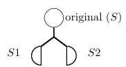
Figure 3.1: A disjoint branching point.
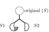
Figure 3.2: A non-disjoint branching point.
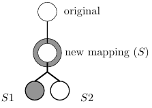
Figure 3.3: Approximation a ects satis ability result.
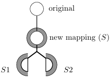
Figure 3.4: Approximation does
not a ect satis ability result.
gray semicircle depicts over-approximated values not present in a precisely modeled predicate shown in Figure 3.1. In the case where a solver cannot precisely model an operation, the symbolic string after the operation will contain additional string values that might a ect reasoning about a branching point, as depicted in Figure 3.3,
or might not, as shown in Figure 3.4. The source of imprecise modeling can be internal to the solver, e.g., as in the
native modeling of substring in EJSA. In addition, it can be the result of improper modeling by the user or the solvers inability to model a string method. Aside from these expected sources, we have encountered an additional source of imprecision, which is inability to represent the full set of characters used in Java. Z3-str only supports a subset of ASCII characters, so we mapped unsupported Java characters to those that Z3-str can handle. This means that multiple Java characters might be mapped to a single character in EZ3-str. Furthermore, we found that STRANGER cannot support at least two UTF-16 charters, one with the decimal value of 0, i.e., a null character, and another with the decimal value of 56319. In this case, the characters are likely restricted due to STRANGERs underlying structure.
Since neither the developers of the four solvers provide formal proofs that their implementations are correct nor we prove the correctness of our extensions, we attempt to evaluate the accuracy of the solvers empirically. The ideal way to experimentally evaluate the accuracy of a solver is to compare its set of solutions for a constraint to the accurate set of solutions. However, since the solution oracle cannot be obtained, we propose nine conservative measurements that can be use to conjecture about solvers accuracy in the context of SE. These measurements are presented in the next section.
3.5 Measurements of Accuracy
We describe these measurements of accuracy so that future users of constraint solvers can adapt their choice measurements when using the solver, i.e., as a means of accuracy evaluation. Furthermore, these measurements may be used in future work on comparison of constraint solvers.
In the following subsections, we refer to two constraint solvers 1 and 2 for use in comparisons of accuracy. We then formally define conditions under which one solver is more accurate than another using the symbol.
3.5.1 Measure 1: Unsatis able Branching Points
Due to complex data and control dependencies between program variables, it is not easy to manually identify feasible and infeasible paths in a program. If all feasible or infeasible paths could be easily identi ed, there would be no need for an analysis
such as SE, but if a constraint solver reports a PC is UNSAT, we can trust the result to be accurate as long as we trust that the constraint solver is sound. Since we assume our solvers are sound, our first measure of accuracy is the number of unsatis able PCs that a solver can detect. If one solver 2 evaluates a constraint as SAT and another 1 as UNSAT, then we say that the latter is more accurate than the former, i.e., 2 unsat 1. The ability of a solver to detect unsatis able PCs is crucial for SE, since it prevents SE from exploring infeasible paths. We refer to the branching points where a solver can detect that one of the outcomes is unsatis able as unsatis able.
We see in Figures 3.1 to 3.4 that before a branching point a symbolic value represents a set of values S. In a constraint solver, the models of opposing predicates will create symbolic values that represent two new sets S1 and S2. An unsatis able branching point indicates that S1 or S2
3.5.2 Measure 2: Singleton Branching Points
Furthermore, in order to assess the complexity of the PCs in unsatis able branching points, we check whether all symbolic string values involved in a branching point contain only a single concrete string value. If this is not the case, then evaluation of the constraint is nontrivial and the unsatis able branching point is marked as non-singleton. Otherwise, we say the branching point is singleton. Therefore, if a solver 1 can detect an unsatis able PC at a non-singleton branching point, then 1 has higher accuracy than a solver 2 that can detect an unsatis able PC at a singleton branching point, i.e., 2 single 1.
Anunsatis able result at a singleton branching point is trivial because the concrete values can be directly used to determine which path is satis able and which is not. In
1 if (s1.equals(“foo”))
2. if(!s1.equals(“bar”))
3. System.out.println(“hello”);
Figure 3.5: A code snippet that demonstrates a singleton branching point and a singleton hotspot.
For an example of both a singleton branching point and a singleton hotspot, consider the code snippet in Figure 3.5. If s1 equals foo at line 1, then a check is performed to see if s1 equals bar at line 2. If it does not, then the program outputs hello at line 3. Because s1 must equal foo in order for a program execution to proceed to line 2, then s1 should only represent a single concrete value, i.e., foo , at line 2. Since the other value involved in the branching point is also concrete, i.e., it is equal to bar , the constraint solver might evaluate the branching point as singleton. Furthermore, because the print statement at line 3 prints the concrete value hello , the corresponding hotspot might also be singleton.
3.5.3 Measure 3: Disjoint Branching Points
The third measure of accuracy evaluates whether or not a solver can partition the domains of symbolic strings at a branching point and directly checks if the second cause of over-approximation described in Section 1.3.3 has produced inaccurate results at a branching point. If the set in the domain of one outcome of a branching point
does not contain values from the set in the domain of the other outcome of the same branching point and vice versa, i.e., if the sets are disjoint, then we say that the solver was able to partition the domain, and it did not over-approximate at that point. We call such branching points disjoint. Conceptually, a disjoint branching point is shown
in Figure 3.1, while a non-disjoint branching point is presented in Figure 3.2. For a more formal de nition, suppose a symbolic value represents a set of strings S, and the two opposing predicates at a branching point separate S into two sets S1 and S2. The branching point is disjoint if S1 S2.
We say that a solver 1 is more accurate than a solver 2 if the set of disjoint branching points produced by 1 is a proper superset of 2 s disjoint branching point set, i.e., 2 disj 1. Note that an unsatis able branching point is a special case of a disjoint branching point.
3.5.4 Measure 4: Complete Branching Points
Similar to unsatis able branching points, we want to identify those disjoint branching points that can add more weight to the evaluation of solvers accuracy, i.e., we want to identify branching points where we know the result is accurate. In general, a disjoint branching point cannot be used to determine whether or not a solver precisely modeled a constraint. For example, if the domain of a symbolic value has been previously over-approximated by an operation or predicate, then such over-approximation may cause a disjoint branching point to become non-disjoint and vise versa. Since we do not prove that models of string operations are precise, we conservatively assume that
none of them are modeled precisely, and we have yet to find a method to empirically disprove this assumption.
Thus, we can only argue that the solver does not over-approximate when a disjoint branching point has never been preceded by either an operation or a non-disjoint branching point. We say this type of disjoint branching point is a complete branching point. A complete branching point indicates that the result of a constraint solver is not over-approximated. For this accuracy measure, we say that a solver 1 is more accurate than a solver 2 if the set of complete branching points for 1 is a proper superset of the same set for 2, i.e., 2 comp 1.
3.5.5 Measure 5: Subset Branching Points
Because di erent solvers use di erent decision procedures, some solvers may be capable of supporting extra measurements of accuracy. For example, an automaton is used to describe a set of strings, so automata-based string constraint solvers are naturally capable of using set operations. This subsection introduces a measure of accuracy that is based on set operations. Since only our automata-based solver extensions deal with sets, this measure of accuracy does not apply to EZ3-str and EECLiPSe-str.
Suppose we have a symbolic value S whose values should be separated into two sets after a branching point, as represented by symbolic values S1 and S2, e.g., S1 represents S after the true branch and S2 represents S after the false branch corresponding to S.contains( foo ). A fth measure of accuracy describes when the
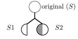
Figure 3.6: A subset branching point that falls under case one.

Figure 3.7: A subset branching
point that falls under case two.
set of values represented by S1 is a subset of the set of values represented by S2, or vice versa, i.e., S1 S2 or S2 S1. These branching points, which we refer to as subset branching points, indicate that the predicate modeled for at least one branch did not change the set of values represented by S, i.e. they indicate that S1 S or S2 S. In other words, if the set in the domain of one outcome of the branching point is a subset of another outcome of the same branching point then we call the branching point a subset branching point.
Conceptually, a subset branching point is shown in Figures 3.6 and 3.7. In these gures, the original set is not constrained by one predicate. Instead, we assign all values in the set represented by the original symbolic value to the domain of the S2 branch, and over-approximated values in the gures are shown in gray. Because the set of values representing the S1 branch is a proper subset of the set of values from the original symbolic value, it is also a proper subset of the set of values representing the S2 branch.
Since the sets in the domains of both branches should contain di erent values, a subset branching point only occurs in a sound solver if the constraints describing one or more branches did not restrict the symbolic value occurring before the branching point. We say that solver 1 is more accurate than solver 2 if the set of subset branching points for 2 is a proper superset of the set of subset branching points for 1. In this case, we say 2 subset 1. Note that unsatis able branching points are a special case of subset branching points, but in our analysis we only measure subset branching points that are not also unsatis able, since we measure unsatis able branching points separately.
There are two cases of subset branching points. Say that in a subset branching point S1 is the subset and S2 is the superset, i.e., S1 S2 S2 S. In the rst case, S1 should be the empty set, i.e., the PC describing S1 should be unsatis able. In this case, if the constraint solver reports that the PC for S1 is unsatis able, it has produced the correct satis ability results. Otherwise, over-approximation has occurred in the solution for the PC describing S1, as we see using the gray shading in Figure 3.7.
In the second case, which is shown in Figure 3.6, S1 should not be the empty set. In this case, over-approximation has occurred in the constraint solvers model for the PC describing S2, and there may be over-approximation in the solvers model of the PC describing S1. In DSE, we can use the path taken during concrete execution to determine if S1 should not be the empty set. If the path for S1 is taken in concrete execution, we know S1 should not be the empty set, so the subset branching point falls under the second case. When this happens, we can conclusively say that the solvers model of the PC describing S2 is imprecise, making its result inaccurate. In our analysis, we do not distinguish the two cases, since we observe interesting results in Chapter 6 without making this distinction. However, future analyses may benefit from separating the two cases.
3.5.6 Measure 6: Additional Value Branching Points
Our sixth measure of accuracy directly tests if the models of the branches at a branching point produce extra values. When the set representing the original symbolic value S is a proper subset of the union of sets from the domains of both branches of a branching point, i.e., S S1 S2, we say an additional value branching point has occurred. An additional value branching point means that a model of at least one branch has produced at least one extra value in its domain of values that was not present in the original set of values. We say that a solver 1 is more accurate than solver 2 if the set of additional value branching points for 1 is a proper subset of the set of additional value branching points for 2, i.e., 2 adval 1.
3.5.7 Measure 7: Top Operations
Our final measure of accuracy addresses operations that a solver is incapable of modeling. When a solver encounters an operation it cannot model, e.g., when EECLiPSe-str encounters replace, the user must approximate the result to be a new symbolic string that represents any string. We say that a top operation occurs when a solver cannot model an operation and the result of a solver that can model the operation is not an unrestricted symbolic value. For example, ESTRANGER cannot model reverse but EJSA can, so if reverse is encountered and EJSA does not produce an unrestricted symbolic value then ESTRANGER has encountered a top operation. Note that if EJSA instead produces an unrestricted symbolic value, then ESTRANGERs result might not have been over-approximated. We call it a top operation because the user must over-approximate the symbolic string value to be the maximum, i.e., top, element in a lattice of symbolic string values. If the set of top operations produced by a solver 1 is a proper subset of the set of top operations produced by another solver 2, then 2 top 1 and 1 is more accurate than 2.
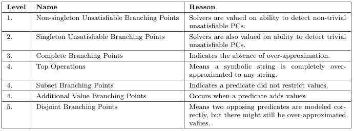
Table 3.2: Displays the importance of each measurement of accuracy.
3.5.8 Hierarchy of Accuracy
We use Table 3.2 to demonstrate the importance of each measurement of accuracy in a solvers overall evaluation of accuracy. In this table, the Level column denotes the level of importance, with lower levels being the most important. The Name column gives the name of the measurement of accuracy, and the Reason column states why that measurement of accuracy falls under that level of importance. For example, we say that non-singleton unsatis able branching points play a bigger role in the overall accuracy of a solver than any other measurement of accuracy, since it has a level of 1 .
We built this table from a SE perspective. In SE, unsatis able PCs are used to identify infeasible paths and show that there are no errors at a program point. Therefore, we place much value on unsatis able branching points. Since non-singleton unsatis able branching points are harder to detect, we place more value on these branching points then singleton unsatis able branching points. We also place value on complete branching points, since they indicate that symbolic values are free from over-approximation. Top operations, subset branching points, and additional value
branching points all de nitely indicate the presence of over-approximation, so we place them in the next level. Finally, disjoint branching points indicate that opposing predicates are precisely modeled, but do not tell whether or not over-approximation exists. Therefore, disjoint branching points are the least important measurement of accuracy.
The user of a constraint solver might place different importance on each measurement of accuracy. We suggest that the user adjust the importance of each measurement of accuracy based on his or her needs. For example, a user might choose to place more importance on complete branching points than unsatis able branching points.
3.6 Dynamically Comparing Solvers
The metrics for comparison presented in the previous sections may be integrated within any tool that makes use of a string constraint solver. We choose to use constraints gathered from real world programs when comparing our extended solvers. Furthermore, we prefer to invoke the solvers as few times as possible. For example, detecting a singleton branching point is simpler if we can obtain a concrete value for each symbolic value in a branching point, instead of querying the constraint solver for such a value.
We use DSE as an analysis technique. DSE is capable of analyzing long and complex program paths gathered from real world programs. In addition, a concrete value can be gathered for each symbolic value at each program point. The advantage to obtaining this concrete value is twofold. First, it can be used to optimize measurements of accuracy such as singleton branching points. Second, it can be used to partially check a constraint solver for soundness. We present more details on such a soundness check in Section 5.4.
However, the main purpose of the next chapter is to introduce our DSE tool, which we use to empirically evaluate our four extended string constraint solvers. After that, we discuss how the above metrics for comparison were integrated within our DSE tool.
CHAPTER 4
STRING SOLVER ANALYSIS FRAMEWORK
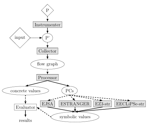
Figure 4.1: Diagram of SSAF.
4.1 Overview
In order to perform empirical evaluation of the extended string constraint solvers, we describe String Solver Analysis Framework (SSAF). The diagram of SSAF is presented in Figure 4.1, which shows a high level overview of the framework from instrumenting a program to recording metrics used in the evaluation. Systemwide inputs are shown in diamonds. The main components of the framework (instrumenter, collector, processor, and each constraint solver) are shown in grey rectangles. Dotted arrows indicate the inputs to these components. The outputs of each component are shown in ovals with solid arrows pointing to them. The white rectangle depicts the evaluator.
SSAF is comprised of the following components: an instrumenter that adds function calls to the program to track string attributes, a collector that uses these attributes to build a CG, a processor that extracts constraints and concrete values from the CG, and extensions to JSA, STRANGER, Z3-str, and ECLiPSe-str, which solve these constraints. The main purpose of SSAF is to perform DSE on an assortment of Java programs and record the constraint solver metrics introduced in Chapter 3. The metrics are measured in the evaluator, which we will describe in detail in Chapter 5.
First, the source code of a program, depicted as the P node in our diagram, is passed to the instrumenter, which compiles the program while adding function calls. Data is passed into the function calls to keep track of useful information, such as string variables, string methods, concrete values, the point in the code where the function was called, and any arguments the string method may have. At this point, the program is instrumented and compiled, and is represented by the Pnode in the diagram.
When the instrumented program P executes on inputs shown as the input diamond in Figure 4.1, the added function calls invoke the collector. The collector collects data and builds a CG based on the data passed in these function calls. When the program terminates, the CG is optimized and serialized in order to be passed to the next component, the processor. At this point, the collector has nished its task of building a CG based on string constraints. A CG produced by the collector takes on a special form, and we call this specialized CG a ow graph (FG), which we define below:
Definition 4.1.
A ow graph is a directed acyclic graph where all source vertices represent either symbolic or concrete values and all remaining vertices represent either operations or predicates encountered during execution. An edge represents the ow of data from one vertex to another. Sink vertices represent functions that consume a particular type of data, e.g., string, but return data of an untracked type, e.g., boolean.
The processor reads in a FG created by the collector, traverses it in a temporal order, and generates PCs based on the vertices in the FG. The processor extracts initial symbolic values, constraints, and concrete values from the FG. Since we do not track boolean values, all string predicates are represented by sink vertices. In addition, we use sink vertices to represent hotspots. When a branching point vertex, i.e., a sink vertex, is encountered, the PC for each branch is passed to the next component, which is a constraint solver. In addition, the PC for each hotspot is also passed to the solver. At this point, the processor has created a PC to be solved by a constraint solver.
Because SSAF uses DSE, which does not require feasibility checks at each branching point, the constraint solvers only solve a PC for evaluation of performance and accuracy. When the solvers solve a PC, the evaluator, which is partially built into each solver, uses the results to record its metrics. This means that the symbolic values produced by each solver, along with concrete values gathered using DSE, are analyzed within the evaluator. Then, the evaluator outputs results used to determine the performance and accuracy of each constraint solver. Once all PCs for a program execution have been analyzed by all four solvers, we have collected our metrics for comparison of the string constraint solvers. Further implementation details of the ins trumenter, collector, processor, and constraint solvers are presented below.
4.2 Instrumenter
Our instrumenter analyzes each statement in a program and takes different actions depending on the type of statement. This section gives a technical description of actions taken for three types of statements. However, we start by explaining how instrumentation is performed. Instrumentation [20] is the process of inserting additional statements into a program in order to track certain program attributes. In our case, we want to track the propagation of string values and string methods throughout the program. In SSAF, the instrumenter uses soot [42] to instrument a program by inserting invoke statements, i.e., function calls, into the program.
Before the program is instrumented, soot rst converts the code into an intermediate representation called jimple that is three-address code. Three-address code is often used in program analysis and compiler optimization, and it represents each statement
n(String s1, String s2){
s1 = s1.concat(“foo”).replace(a, b);
if (s1.equals(s2) || s2.contains(“bar”)) {
…
Figure 4.2: Example demonstrates multiple address code.
n(String s1, String s2){
String temp1 = s1.concat(“foo”);
s1=temp1.replace(a, b);
boolean a=false;
if(s1.equals(s2))
a=true;
if(s2.contains(“bar”))
a=true;
if(a){
…
Figure 4.3: Demonstrates three-address code.
in a simpler form using one assignment and two operands. For example, consider the code snippet in Figure 4.2. The code features multiple operations (concat and replace) in one line that modi es variable s1 and multiple comparisons (equals and contains) in its branching point. Notice that this codes representation is semantically equivalent to the three-address code representation presented in Figure 4.3. This representation reduces the complexity of instrumentation by considering each string method independently, instead of considering combinations of methods. Upon encountering an assignment statement, e.g., a = b, the instrumenter checks if the variable type on the left hand side (LHS) is a string. If so, an invoke statement that captures the ow of the right hand side (RHS) to the LHS is inserted into the program either immediately before or after the statement. In the CG, this ow of data is captured by an edge from the vertex of the RHS to the vertex of the LHS. If the RHS is an invoke expression, e.g., s1.concat(s2), extra steps are taken.
When a string invoke expression, or an invoke expression representing a hotspot, is encountered either on the RHS of an assignment statement or as an invoke statement, the instrumenter inserts invoke statements that add an edge in the CG from the vertex of each argument to a vertex representing the invoke expression itself. These invoke
statements are inserted immediately before the invoke expression. If the calling string is a StringBuilder or String Buffer, an invoke statement that adds an edge from the invoke expression to a new vertex for the calling string is also inserted. This is because these classes represent mutable string types. This edge is also added if the string variable is the target of a modi cation, e.g., for s1=s1.trim().
These two types of statements cover the basic functionality of the instrumenter. However, additional record keeping must be added to account for function calls within a program. For example, if a function foo that contains a string parameter and returns a string is called in a main method, then we want to record the ow of data from the argument to foo s parameter. In addition, we want to record the ow of foo s string return value back to the main method. This is done by adding an invoke statement that is called with every occurrence of a string parameter or string return statement. This process is fairly straightforward; however, interprocedural DSE creates challenges.
To address these challenges, we record a stack of method calls to ensure that we pass and return values in the proper order. The instrumenters role in this task is to identify entry and exit points of each method then add a collector function that marks the entry or exit of that method. In order to correctly represent the behavior of di erent types of program variables, the variable types are differentiated within the intrumenter and collector. For example, each variable can be a field reference, a static field reference, a parameter, a
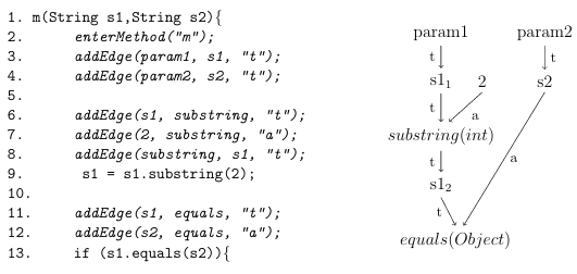
Figure 4.4: Instrumented code and the corresponding CG. Based on code in Figure 2.1.
return variable, or a local variable, and the collector performs a di erent action based on this type. In addition, a program variables type can come from any Java primitive or Java class/interface. A variable that has a non string type is only tracked as an argument to a string method, so we only record the ow of data for string variables, i.e., variables of type String, StringBuilder, or StringBuffer. To demonstrate the e ects of our instrumentation, consider the code snippet and CG in Figure 4.4. This snippet is based on the code in Figure 2.1, and the instrumented lines are in italic. In this example, line 2 contains the invoke statement that informs the collector that the m method is entered. Lines 3 and 4 define the variables s1 and s2 to be parameters. The collector later uses this information to
optimize the CG. Lines 6-8 create the edges leading to and from the substring method. Note that lines 6 and 7 capture the substring invocation while line 8 captures the assignment statement. Lines 11 and 12 create two edges that lead to the equals method, one for the calling string (labeled t for target) and one for the argument (labeled a ).
Figure 4.4 also shows a unoptimized CG that might be generated while executing the code snippet. This CG is similar to the one in Figure 2.2, but it contains parameter labels and string variable values instead of symbolic values. Notice that there are two vertices for s1: s11 and s12. These vertices re ect two separate values given to s1. s11 is an initial value while s12 is s1s value after the substring(int) operation.
This example shows the instrumenters general approach. In addition, it shows the overhead required to run an instrumented program. We added several method calls for each string method, which in turn adds several edges to the CG. The snippet from Figure 4.4 is only used for a demonstration and does not reveal the instrumenters overall complexity. For example, we add arguments describing the variable type and the concrete value of the variable for that execution into the collectors addEdge method. After all statements have been traversed, a shutdown hook is added that prompts the collector to optimize and serialize the CG. The optimized CG resembles the one in Figure 2.2. This shutdown hook is called immediately before the program exits.
4.3 Collector
The collector contains several static functions called throughout the execution of the program. The main collector function, i.e., the addEdge function that we demonstrated in Figure 4.4, adds an edge to the CG at the appropriate time. All vertices are stored in a map for easy retrieval when the corresponding variable is used again. Each vertex contains the method or variable name. A vertex also contains a concrete value that was given in the instrumented method and a unique id that increases with every newly created vertex. When an existing edge is added again, a
new target vertex is created to preserve values. This step prevents the creation of cycles, which make it di cult to traverse the graph.
In order to x the aforementioned problems with interprocedural analysis, a call stack for each method in the program is maintained. Then, only the vertices for the call stack level of a particular method are loaded. Therefore, a stack of maps (of vertices in the CG) is maintained. When a new method in the program is entered, a new map is created at the top of the stack. When the method is exited, the top map of the stack is popped.
After the instrumented program nishes execution, i.e., when the shutdown hook is called, we collapse redundant vertices in the CG. For example, we collapse the s12, param1, and param2 vertices from the CG in Figure 4.4 to generate the CG in Figure 2.2. We need these vertices to track dependencies when building the CG, but since we are only interested in the ow of data, we dont need these vertices in the nal FG.
We only need vertices representing concrete values, initial symbolic values, operations, predicates, and hotspots. Therefore, these vertices are removed and outgoing edges are adjusted to originate from the source of the incoming edges. All remaining vertices depicting variables, e.g., s11 and s2 in Figure 4.4 are now treated as symbolic values. After these optimization steps, the CG is a FG, and we serialize it in order to pass it to the processor.
4.4 Processor
The purpose of the processor is to traverse a serialized FG to create PCs and to send these PCs to the constraint solvers. The CG is processed in a temporal breadth first search order. That is, the processor always removes the oldest source vertex (based on the unique id) remaining in the graph. The processor di erentiates original source vertices, internal vertices, and sink vertices when passing them into a constraint solver so that the solver knows that the vertices should be respectfully treated as initial symbolic or concrete values, operations, or predicates. The processor contains an interface to each extended string constraint solver, which we introduce next.
4.5 Constraint Solvers
A constraint solver in SSAF is an extension of a publicly available constraint solver and is implemented through a Java interface with three primary methods that are called by the processor: add Source, add Operation, and add Sink. This is done on an intermediate level so that the underlying constraint solver can be adapted to solve constraints speci c to the Java language. Constraint solvers are not language specific, but that means most of them do not provide trivial representations of many Java Application Programming Interface (API) functions, e.g., trim(). In addition, they each need to be adapted for use with SSAF. Note that the implementation of each string method varies based on the underlying constraint solver. However, each implementation performs the same basic tasks. add Source is called whenever a new symbolic value or concrete value is created. If the value is symbolic, it represents any value. Otherwise, the value is hard coded into the program, so it should only be represented by that one value. All variables that are not of string types, e.g., integer variables, are assigned their runtime values that were gathered during DSE.
add Operation is called whenever a symbolic value is modi ed. For example, an integer symbolic value I might by modified by I = I + 1 whereas a string symbolic value S might by modi ed by S.append(1). These modi cations are added to the PCs.
A constraint solver does not have to evaluate PCs at these points, but these operations certainly a ect the outcomes of future PCs. addSink applies assertions made by predicates and checks for soundness and accuracy. These checks essentially make up the evaluator in Figure 4.1. First, the constraint solver checks if a sink vertex is a predicate. If it is a predicate, then different metrics are measured and assertions are made on the arguments of that predicate based on the actual outcome. Because predicates are represented as sink vertices in the FG, assertions made on the predicate itself are useless for future evaluations of predicates and hotspots. Therefore, assertions are made on the arguments of each predicate. For example, we know a string symbolic value S is equal to foo if the outcome of S.equals( foo ) is true and should not equal foo if the outcome is false.
The processor does not di erentiate the methods encountered, e.g., it does not know if it passed an append or a substring operation to a constraint solver. Although that approach is viable, we instead allowed each solver to make this differentiation. We did this for two reasons. First, it would be tedious to make this distinction within the processor. Second, there are several methods that require the same action from the solver, e.g., append is overloaded to accept several di erent variable types when it has one argument, but it does the same thing regardless of the type. In addition, the processor does not di erentiate the methods class because the same action is taken regardless of the class, e.g., substring(int) appears in all three string classes but does the same thing regardless of the calling class.
We describe implementation details speci c to each solver below. This includes descriptions of several string methods for each solver. However, there are several methods that are modeled in a similar way by each solver. For example, toString, valueOf, intern, trim To Size, and copy Value Of involve propagating a symbolic value.
For methods such as these, we do not reiterate the approach taken within each solver. Each solver also takes the same basic approach when modeling operations such as setCharAt, insert, delete, and deleteCharAt. We demonstrate this approach by explaining our model of insert(int,String), which inserts a String value into a StringBuilder or StringBuffer variable at the location specified by the integer argument.
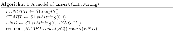
We show our approach at modeling insert(int,String) in Algorithm 1. In this algorithm, S1 is the symbolic string representing the calling string, i is the first argument, which takes a concrete integer value, and S2 is the symbolic string representing the second argument. Notice that LENGTH is a symbolic integer representing S1s length, START represents the start of the calling string, and END represents the end of the calling string. This model returns a symbolic string representing the calling string with the symbolic string for the second argument inserted at the location specified by the first integer argument. First, the beginning of the symbolic value representing the calling String Builder or String Buffer object is extracted using the integer argument along with the substring operation. Second, the end of the symbolic value is extracted in a similar way. Finally, the beginning of the symbolic value is concatenated with the symbolic
![]()
Figure 4.5: Nodeterministic automata that were independently created by extracting the first two and last character of the string foo .
Figure 4.6: Nodeterministic automaton representing foo after bar has been inserted at index 2.
string argument, and the result is concatenated with the end of the symbolic value extracted using the substring operation. SetCharAt is similar, but the argument is a single character and a character is excluded from the beginning substring. Delete and delete CharAt do not add anything between the extracted beginning and end of
the calling string. We demonstrate an automata example of our model of insert(int,String) using Figures 4.5 and 4.6. When constructing these automata, we assume the method foo .insert(2, bar ) was called. Figure 4.5 shows the automata representing the beginning and ending substrings of foo , which have been separated by the substring operation at the second index to respectively represent fo and o .
Remember that the original automaton for foo is shown in Figure 2.4. These substrings were extracted in the rst and second step of our insertion algorithm. In the third step, we insert the bar automaton between the two substrings using concatenation operations. The result is shown in Figure 4.6. Whenever a solver cannot model an operation, we over-approximate the result to be any string, i.e., we return the top element in a lattice of symbolic string values. For example, only EJSA can model reverse. If a solver cannot model a predicate, we over-approximate the result to be the original symbolic value occurring before the predicate, i.e., we do not constrain the original symbolic value. For example, if a solver cannot model the not equals predicate for s1.equals(s2), we simply do not perform any action when encountering that method.
In particular, we do not model any hybrid constraints. A hybrid constraint requires a constraint solver that solves constraints from multiple theories, such as string and integer theory. For example, the charAt method requires a comparison to a character to assert a constraint on the calling symbolic value. Because we only track string types, we cannot determine if this comparison is performed in the program and opt not to collect the concrete solution using DSE. The solvers we extended are capable of modeling some hybrid constraints, but we chose to conduct our comparison of string constraint solvers on pure string constraints. Future work may focus on comparisons of hybrid solvers. When evaluating a PC, we only consider the variables involved in the branching point. For example, a variable s1 might be in the PC when we evaluate s2.equals(s3), but we do not send any queries related to s1 when evaluating the method because we already know we must have a satisfiable assignment for s1 to reach that point. We
therefore decompose the query based on variables used at a specific program point.
Table 4.1 shows the basic operations and predicates used for each extended solver. The rst column names the operation or predicate. The second gives a brief description. The nal four columns tell if the operation or predicate is respectively available using an x mark for EJSA, ESTRANGER, EZ3-str, or EECLiPSe-str. Even though the basic operation or predicate may not be available, we may model it using available interfaces, e.g., as was done for insert(int,String). Moreover, some operations and predicates require additional overhead to be viable for our analysis. For example, trim requires unexpected e ort in modeling for EJSA and
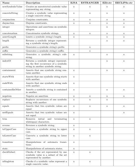
Table 4.1: Available inter faces used in the extended solvers.
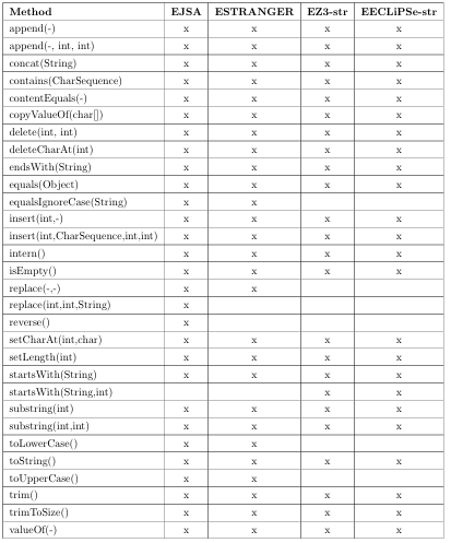
Table4.2: Describes the method s modeled by each extended string constraint so lver.
ESTRANGER, as we explain below. In order to characterize what these basic operations and predicates can do, we list all Java string methods that we modeled in Table 4.2. The rst column gives a method signature, while the remaining four columns use an x to respectively indicate if that method is modeled in EJSA, ESTRANGER, EZ3-str, or EECLiPSe-str. Recall that one method could occur in multiple string classes, e.g., substring(int) is in all three
string classes. We represent all overloaded methods using the wildcard character- in method signatures, e.g., replace(-,-) denotes both replace(char,char) and replace(CharSequence, CharSequence). Whenever we omit a description of a model for a method in Table 4.2 while explaining the implementation details of a solver, it has a direct mapping from an operation or predicate in Table 4.1. Not all of the methods in Table 4.2 were encountered in our experiments. We chose to implement extra methods in all of our extended solvers. This was done to make the solvers more diverse and to investigate challenges in implementing these extra methods. The remainder of this chapter addresses implementation details for each solver.
4.5.1 EJSA
JSA was initially built to model Java string methods in static analysis. Therefore, it comes with several built in models of Java methods. However, JSA still required several adaptations for use in SSAF. For example, we discussed a reimplementation of the substring method in Section 3.1. The rest of this subsection describes other implementation details for EJSA. When we initially ran performance experiments, we found that the first predicates and operations encountered required a large amount of time to solve, i.e., JSA incurred a startup time. This appears to have been caused from lazy loading of the underlying library and was xed by preloading JSAs methods.
We chose to use our own implementation of set CharAt, insert, delete, and delete CharAt based on our more accurate models of the substring operations and the insert(int,String) model in Algorithm 1, even though JSA does provide its own interface for these methods. We believe the previous example of insert(int,String) is more accurate than JSAs native modeling of insert(int,String), which over-approximates the result to allow the argument to be inserted at any point within the calling symbolic string. JSAs native approach was effective for its intended analysis, which did not track the values of integer arguments. Instead of using this native approach, we opted to use the information gained from DSE to improve the accuracy of EJSA, as well as the other solvers.
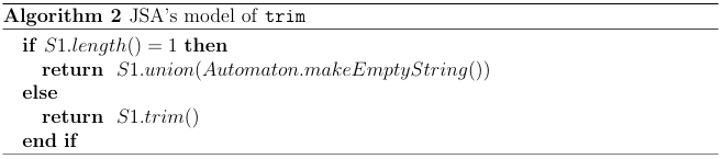
JSAs trim implementation contains an error, i.e., there is a case where an unsound result is returned. This occurs when the calling automaton represents a single concrete string with one character, e.g., the concrete string a . In this case, JSAs trim interface will return an automaton representing the empty language instead of the original concrete string. To x this bug in EJSA, we check if the original automaton represents a string of length one. If it does, then we over-approximate the result to be that automaton disjoined with an automaton representing the empty string. Otherwise, we apply JSAs trim operation. We show our approach in Algorithm 2.
In this algorithm, S1 is the automaton representing the calling string. Notice that S1.length() returns a symbolic value, but we compare it to the concrete value 1. This comparison returns a true result when the symbolic integer only represents a single concrete integer. In addition to the aforementioned operations, we modeled several predicates in EJSA. JSA does contain an interface for not contains, but we opted to use a reimplementation since we believe it is more accurate. Not starts With and not ends With were not implemented in JSA because it is di cult to precisely model these predicates in the general case using automata. To demonstrate this di culty, consider the following constraint is passed to JSA:
!(S1 startsWith( foo concat(S2))) (4.1)
In this constraint, S1 and S2 are unrestricted symbolic values representing any string, and JSA uses automata to represent S1 and foo .concat(S2). The not startsWith predicate states that the calling string cannot start with the argument. In the case where the argument is a concrete string, we model the predicate by restricting the values of S1s automaton so that they cannot start with that calling string. However, in the case from Equation 4.1, there is no way to tell which value should be restricted without considering all constraints in the PC. Initially, we attempted to model this constraint by restricting the values of S1s automaton so that its set of strings cannot start with foo , but this model is unsound. To demonstrate why it is unsound, consider that S1 could represent foo and foo .concat(S2) could represent foobar . These concrete assignments follow the path described by the constraint in Equation 4.1, but S1s automaton no longer represents foo because it can no longer start with foo .
Therefore, the automaton is unsound, and in any case where the argument does not represent a single concrete value, we must over-approximate the predicate so that it does not restrict S1s automaton at all. Similar arguments can be used to demonstrate that the models of not equals, not contentEquals, not equalsIgnoreCase, not contains, and not endsWith are difficult to model precisely using automata in the general case. However, these predicates can be precisely modeled by tracking dependencies and restricting symbolic values using these dependencies. This has been done using multi-track automata [49] and a list [37] to track dependencies. Typically, automata-based string constraint solvers do not take such an approach because of the e ort required to track these dependencies, as well as the resource and performance cost of tracking dependencies. Because Z3-str and ECLiPSe-str take the entire PC into consideration instead of incrementally solving constraints, they better record the dependencies required to model these predicates.

We demonstrate our approach at modeling these negated predicates using not contains as an example, and we show this example in Algorithm 3. In this algorithm, S1 represents the calling symbolic string and S2 represents the argument. Because we do not track all of the dependencies between automata, we can only precisely

Figure 4.7: Nondeterministic automaton representing foo after ignore case operation.
model this predicate in an automata-based solver when the argument represents a concrete string. In this case, we create a symbolic string Atemp representing any string, i.e., ANY in Algorithm 3, concatenated with the argument concatenated with any string. After that, we return the intersection of the calling symbolic string with the complement of Atemp. Note that a similar approach is taken with not startsWith and not endsWith, but in these cases Atemp either does not start or end with any string. In a model of not equals and not contentEquals, Atemp is simply the argument.
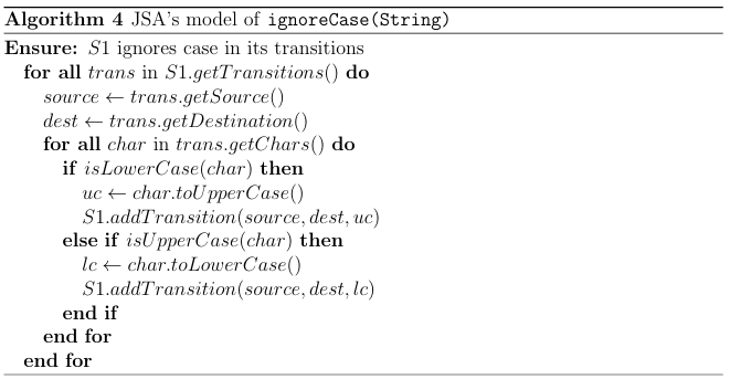
We also added custom models of equals Ignore Case and not equals Ignore Case. These models require an ignore Case operation on the argument, which is shown in Algorithm 4. In this algorithm, we first iterate over every character in every transition
in the argument, which is symbolic string S1. If a character is a lower case character, we add a transition to S1 representing its upper case version, and vice versa for an upper case character. The resulting automaton accepts any string that the original automaton does with any permutation of upper case and lower case letters. We see such an automaton in Figure 4.7, which is the result of applying this ignore Case operation to the foo automaton in Figure 2.4. After applying this operation, we simply apply JSAs equals or not equals predicate.
The above models of predicates neglect to describe constraints on each methods arguments. For example, in S1.contains(S2), we can impose a constraint on S2 stating that it must be a substring of S1. Since our automata-based string constraint solvers require independent operations on each automaton representing a symbolic value, these constraints must be separately enforced, although EZ3-str and EECLiPSe-str naturally enforce these constraints. We make our best e ort to model constraints on the arguments. For example, we constrain the argument to be equal to the calling value in S1.equals(S2). However, in some instances, we must apply weak constraints on the arguments. For example, to model not contains, we only assert that the argument is not equal to the calling string when the calling string only represents a single concrete value.
Future work can determine how to better model these constraints and can determine how to measure the accuracy of constraints on arguments in automata-based solvers. We now proceed to present challenges in extending STRANGER.
4.5.2 ESTRANGER
STRANGER was originally designed to find and eliminate vulnerabilities in PHP programs, and it now works to eliminate these vulnerabilities in several languages.
Therefore, the interface is not tailored speci cally for Java strings. Yet, STRANGER still has a simple interface for many Java string methods that we used in ES TRANGER.
STRANGER is written in C and uses Java Native Access (JNA)1 to allow Java to access the C library. When we obtained STRANGER, it lacked several JNA calls, such as those to the C prefix and suffix functions. We therefore had to write several extra calls. We plan to contribute to STRANGER by adding these calls for future users.
We found that STRANGER has poor support for null and empty strings. This might be caused by either STRANGERs BDD representation of transitions or perhaps from Cs poor model of the null string. To circumvent this issue, we
use STRANGERs make Empty String() method to represent the null string and make Any String L1ToL2(int,int) with 0 as both arguments to represent the empty string.
We also noticed that STRANGER exhibits poor performance in some situations, i.e., with very large automata containing over 5,000 transitions. This is likely caused by its underlying BDD representation of transitions. To x the problem, we replace the result of an operation with an automaton representing any string whenever the number of transitions in the calling automaton or an argument automaton grows to over 5,000. Fortunetely, this rarely happens. Substring(int,int) was derived using STRANGERs built in prefix and suffix operations. Using these prefix and suffix operations, we were also able to use the approach described in Algorithm 1 to model insert, setCharAt, delete, and deleteCharAt. STRANGERs trim interface only trims a single character at a
1https://github.com/twall/jna
time, so we extended it to handle all of Javas whitespace characters as is done in Javas trim method by iteratively trimming each of the aforementioned characters until an iteration no longer changes the automaton.
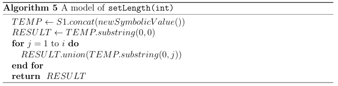
We show ESTRANGERs model of setLength in Algorithm 5. In this algorithm, S1 is the calling symbolic string and i is the integer argument. SetLength is modeled by concatenating the original automaton with an automaton representing any string then returning an automaton accepting any substring of the result up to the given length that starts at index 0, i.e., the pre xes. In ESTRANGER, equals, contentEquals, contains, startsWith, and ends With are all handled in a similar way as EJSA. For example, contains is modeled by intersecting the calling string with automaton Atemp representing any string concatenated with the argument concatenated with any string. The contains algorithm is the same algorithm shown in Algorithm 3, but we do not need to first check if the argument represents a concrete string or compute the complement of Atemp.
Through communication with the developers of STRANGER, we were successfully able to model equals Ignore Case and likewise not equals Ignore Case when the argument represents a concrete string. This is done by creating an automaton that accepts both the upper case and lower case version of each character in the concrete string, as presented in Figure 4.7. EJSAs version of this operation is more robust than ESTRANGERs version in that it allows the argument to represent any symbolic string. Despite that, this model demonstrates the value in communicating with developers and exerting more e ort to model more methods.
EZ3-str and EECLiPSe-str can use a similar approach to model equalsIgnoreCase, but they require more computational e ort because it is dificult to determine if a symbolic value represents a single concrete value in these solvers, since they have no Java API. The approach requires several time consuming queries to the underlying constraint solver, so we opted to sacri ce accuracy for performance. We now proceed to discuss implementation details for EZ3-str.
4.5.3 EZ3-str
Z3-str is currently only available as a standalone program. Therefore, in order to use EZ3-str, we rst convert our PCs into Z3-str syntax. Then, we execute the standalone program. Z3-str can require a long time to solve some PCs because solving string constraints is in general an undecidable problem [5], and is NP-complete for simple fragments of string theory [21]. Thus, we also include a mechanism for creating a timeout for Z3-str.
To execute Z3-str queries, we rst convert each constraint in a PC into Z3-str syntax and write the PC to a le. Whenever we query Z3-str for a solution, we run it with the text le corresponding to a speci c PC. To timeout Z3-str, we kill the process that runs it. This timeout is set to ve seconds. If a timeout occurs in EZ3-str or EECLiPSe-str while checking a PC for satis a bility at a branching point, we exclude that branching point from comparisons. Since
we know the path taken in DSE is feasible, this only happens when we check the negated path for satis ability.
Since we also instantiate Z3-str and ECLiPSe-str to record our measurements of accuracy, a timeout might also occur when recording these measurements. If this happens, we assume the worst accuracy at that branching point for that particular measurement. For example, if a timeout occurs when attempting to detect a singleton unsatis able branching point, we assume the branching point is singleton, as non-singleton unsatis able branching points have better accuracy than singleton unsatis able branching points. One complication in evaluating the performance of EZ3-str is its startup time. We do not want to include this time, which is required to load/initialize Z3-str, in our
performance comparisons, so we exclude this startup time in EZ3-str using Z3-strs self reported time.
This adds a potential internal threat to validity, since we measure EZ3-strs performance using a di erent technique than in the other extended solvers. In the other solvers, we use our own timers, while in EZ3-str we use the timer from the underlying solver. This likely causes EZ3-strs to underreport its time. However, we do not believe that this a ects our conclusion for Section 6.2. Z3-strs interface allows us to model operations such as insert, setCharAt, delete, and deleteCharAt using the technique introduced in Algorithm 1. Just like in ESTRANGER , we model set Length using Algorithm 5. Trimis over-approximated by allowing the result to be any substring of the calling string. Unfortunately, we could not model toUpperCase, toLowerCase, or replace. Even though Z3-str does have a replace interface, it is not suitable for modeling Javas replace methods. Negated predicates such as not equals and not contains were modeled by negating the positive version, e.g., not equals is modeled by negating equals.
Starts With, not startsWith, endsWith, and not endsWith were modeled using the same technique used in ESTRANGER, which is similar to Algorithm 3, only Z3-strs string type is used instead of automata. Note that this means that not startsWith and not endsWith are only asserted when the argument is a concrete value. EZ3-str does not have an interface to check if the argument is a concrete value, but we can track if the argument is an initial concrete value, i.e., a concrete source vertex in our FG. We did try an alternative model for these two predicates, but we found that a timeout occurred often with this alternative model. This alternative model is used in the final version EECLiPSe-str, and the timeout results are re ected in our empirical comparisons of accuracy. We now proceed to discuss this and other implementation details of EECLiPSe-str.
4.5.4 EECLiPSe-str
ECLiPSe-str does not feature a direct Java API. However, the ECLiPSe framework does provide the means to query an instance of ECLiPSe-str that exists in a separate process, so we use this feature in EECLiPSe-str. This requires again converting PCs into a special format, i.e., ECLiPSe-strs input syntax, then running the result as a query. We also had to implement a timeout in EECLiPSe-str. To execute this timeout, we simply terminate and reinitiate the process running EECLiPSe-str. Because we chose not to measure startup time, we do not record the time required to start a new instance of ECLiPSe-str in a new process. Again, the timeout is set to ve seconds. As we mentioned before, substring(int) over-approximates because ECLiPSe strs substring operation must return a string of at least length one. Operations such as insert, setCharAt, delete, and deleteCharAt were modeled using the same techniques used in Algorithm 1. SetLength used the approach in Algorithm 5, and trim was modeled using the same techniques used in EZ3-str. Just like EZ3-str, EECLiPSe-str could not model toUpperCase, toLowerCase, or replace.
In order to model, contains, not contains, startsWith, not starts With, ends With, and not endsWith in EECLiPSe-str, we used the indexOf operation along with symbolic integers. For example, to model contains, we asserted that the return value of indexOf was not 0, which in ECLiPSe-str means that the argument is not present in the calling string. In order to assert endsWith and not endsWith, we had to calculate the symbolic lengths of the calling string and the argument using ECLiPSe-str. We directly used ECLiPSe-strs length, equality, and negation operations to model is Empty, not is Empty, equals, not equals, content Equals, and not content Equals.
4.6 Summary
This chapter presented the overall design of our DSE framework, SSAF, along with specifics on how the extended solvers model several Java string methods. Note that this is one of several potential designs for such a tool, and there may be better ways to implement several models we described for our solvers. Even though the implementation details we described above are important for a string constraint solver user, the main purpose of our thesis is to highlight the different metrics that are important for constraint solvers of complex types, i.e, performance, accuracy, and modeling cost. Thus, this chapter provided implementation details of SSAF and the next chapter details how to empirically measure the metrics described in Chapter 3.
CHAPTER 5
THE EVALUATOR
In this chapter, we describe the evaluator shown in Figure 4.1, which actually performs the comparisons of string constraint solvers. We also explain in detail how we collect data for comparison of our extended string constraint solvers using SSAF. We intentionally separate this chapter from Chapter 3 in order to keep definitions separate from implementation. Furthermore, we chose to introduce SSAF before describing how we use it for comparisons. This chapter should be separate from Chapter 4 because comparisons based on our metrics can be made in any analysis tool that uses constraint solvers, not just SSAF. We evaluate the solvers using the following categories: performance, modeling cost, and accuracy, which are important metrics for the user of a constraint solver.
5.1 Performance
EJSA and ESTRANGER are both incremental constraint solvers. Recall that an incremental constraint solver is capable of remembering solutions from previous PCs in order to solve future PCs. To compare these solvers with non-incremental solvers, we must incrementally measure performance. For our automata-based solvers, this is done by storing the time required to create an automaton, along with the automaton, using a timer. If previous automata are used in an operation or predicate, we collect the time required to create the automata and add the time required to impose the additional operation or predicate.
Calculating the time required to solve a PC is simpler in EZ3-str and EECLiPSe str than in the automata-based solvers. We measure the total time required for the solver to solve a query or timeout. This is done by starting a timer immediately before the query is submitted and stopping it when the query is returned or when a timeout occurs.
We believe that both of these approaches provide a consistent means of determining performance among the solvers. In order to capture the solvers performance on a wide array of PCs, we record the time required to solve the PC for each branch at a branching point, i.e., we record the time required to solve the PC for the branch taken in DSE in addition to the one not taken. To ensure that the performance results are comparable, we calculate the average time for each program trace. To better describe the characteristics of time required to solve PCs, we also determine the median time required to solve PCs at branching points.
5.2 Modeling Cost
In our comparison, we use the LOC required for us to extend a solver to model each method as the measure of modeling cost. Although the more objective measure would be the amount of time we invested in extending each solver, we believe that the number of LOC is representative of the overall e ort. This count of LOC does not include the xed cost required to extend each constraint solver. For example, it does not capture the task of determining the arguments for a string method or how we set up Z3-str and ECLiPSe-str to run in a separate process. We only measure the variable cost, which changes based on the methods implemented, as well as the precision of their models. We use this variable cost to compare the modeling e ort in terms of each method, since we believe the accuracy of a method is dependent on the modeling cost for that method. On the other hand, the xed cost is the same no matter what methods we choose to model in a particular extended solver.
5.3 Measurements of Accuracy
The measurements of accuracy discussed in this section relate to those presented in Section 3.5. However, whereas that section de nes each measurement, this section describes how SSAF can be used to measure each of them.
5.3.1 Measure 1: Unsatis able Branching Points
Unsatis able branching points can only be recorded for negated branches from those taken in DSE, i.e., one negated branch per branching point, because the path taken in DSE is always satis able. Therefore, we look for an unsatis able branching point by querying a solver with the PC representing the negated branch at a branching point. The satis ability results are then recorded for the solver. For the automata-based string constraint solvers, an unsatis able result occurs when an automaton represents the empty language, so a test on the emptiness of an automatons language is used to determine satis ability. On the other hand, Z3-strand ECLiPSe-str directly report satis ability results when a query is submitted.
5.3.2 Measure 2: Singleton Branching Points
A singleton branching point is calculated by rst collecting a concrete value for each symbolic value in a PC. In a static analysis, these values would have to be collected by querying the solver. However, because we use DSE, we collect the concrete values from the programs execution. After that, a constraint for each symbolic value is independently conjoined with the PC and the solvers are queried with each resulting conjunction of constraints. The independent constraint states that the symbolic value cannot equal the concrete value we collected. If the result is UNSAT, then the symbolic value can only represent the concrete value we collected. Otherwise, the symbolic value can represent several concrete values. Note that in order for a branching point to be a singleton branching point all symbolic values involved must correspond to one concrete value, so we separately determine the values represented by each symbolic value.
5.3.3 Measure 3: Disjoint Branching Points
A disjoint branching point occurs when there is no overlap in the sets of values from the domains of both branches of a branching point. A disjoint branching point may therefore be detected if we attempt to find the overlap and instead find that there is none. This overlap happens to represent the values that occur when both branch outcomes are true. Therefore, we can detect a disjoint branching point by creating a constraint indicating that both branches were taken and querying the solver with that constraint. If the result is UNSAT, the branching point is disjoint. Otherwise, it is not disjoint. This constraint is created by simply conjoining the PC for one branch with the predicate describing the other branch. For example, since automata-based solvers can use the intersection operation to denote conjunction, a disjoint branching point for an automata-based solver may be dectected by intersecting the two automata that represent both taken branches.
5.3.4 Measure 4: Complete Branching Points
A complete branching point is a disjoint branching point that we know has not been preceded by over-approximation. When measuring these branching points, we error on the safe side by conservatively identifying sources of over-approximation to be either operations or non disjoint branching points. We do this because a disjoint branching point is the only type of branching point that we know has been modeled precisely, and we have yet to empirically determine if an operation is free of over-approximation. The only challenge that remains is to track the propagation of potential over approximation. For example, if a non disjoint branching point is followed by two disjoint branching points, we cannot rely on the accuracy of the two disjoint branching points. In order to track this over-approximation, we use a taint analysis, where the taint source is any potentially over-approximated branching point or operation.
The result of any branching point or operation that involves at least one tainted value is also marked as tainted. We can trust any singleton branching points to be free of over-approximation, so taint is removed when a branching point is a singleton branching point. With that said, when a branching point is disjoint and all values involved are free of over-approximation, i.e., the values are not tainted, that branching point is also complete.
5.3.5 Measure 5: Subset Branching Points
We previously mentioned that only our extended automata-based solvers are capable of detecting subset branching points. In order to detect one of these branching points in an automata-based solver, we calculate the two automata representing both branch outcomes. We then use a built in method in both JSA and STRANGER to determine if one branch outcome automaton is a subset of the other and record the result.
5.3.6 Measure 6: Additional
Value Branching Points We can also check if an automata solvers model of a branch adds extra values to the set represented by the symbolic value occurring before the branching point using JSA and STRANGERs built in method to detect proper subsets. This is done by disjoining the two automata representing the two branch outcomes and checking if the automaton occurring before the branching point is a proper subset of the result.
5.3.7 Measure 7: Top Operations
There are two criteria that must be met in order to record a top operation. First, a solver must not be able to handle an operation and we must approximate the result as any value. Second, a second solver that can handle the operation must report that the symbolic value should not represent any value. If the second solver reports that the symbolic value should represent any value, then the operation did not cause over-approximation.
The first criteria is met in any solver by simply reporting when an operation that a solver cannot model has been encountered. However, the second criteria can only be met by EJSA or ESTRANGER, since they allow us to check if a symbolic string
represents any value and the other two solvers do not. When any solver encounters an operation it cannot handle and EJSA or ESTRANGER reports that the symbolic string should not represent any value then a top operation is recorded for the solver that could not handle the operation. Since we are only capable of using EJSA or ESTRANGER to check if a symbolic value should represent any value, there is a potential internal threat to validity in our measurement of top operations against EZ3-str and EECLiPSe-str. To remove this threat, we only record top operations for EZ3-str and EECLiPSe-str. Even though we are not comparing top operations for all of our solvers, they are still useful because they show that over-approximation has occurred.
5.4 Debugging
Up until this point, we have discussed the evaluator with regard to evaluating string constraint solvers. However, we also used the evaluator for debugging throughout development of SSAF. Therefore, we include this section to detail how we used soundness and completeness checks to help verify that our extended solvers were implemented correctly. The developers of the string constraint solvers do make claims to the soundness of their solvers, and we make our best e ort to guarantee soundness in our extended solvers. However, the developers do not provide formal proofs of the soundness of their solvers, and we do not formally prove the soundness of our extensions. For this reason, we use two techniques to verify that the extended solvers are at least partially sound. For the first, we gather a concrete value for each symbolic value at each branching point. Then, we check that each concrete value is represented by its
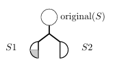
Figure 5.1: An unsound branching point.
symbolic value for the respective variable at that program point. This is only possible because we use DSE for our comparisons instead of a static technique. Essentially, we use DSE as an oracle to collect values that we know should appear given the PC and debug the extended solvers based on these values. For the second partial soundness check, we directly check if the model of the branches at a branching point are unsound, i.e., we check if some solutions are lost in a model of a branch. If the union of sets from the domains of both branches of a branching point is a proper subset of the set of values represented by the original symbolic value occurring before the branching point, then the constraints generated to model the branches removed some values from the set represented by the original symbolic value, and at least one model is unsound. Conceptually, this can be pictured in Figure 5.1. In this gure, missing values that should be present in the S1 branch but are not are shown in light gray. Essentially, this check ensures that each value represented by the original symbolic value is present in the domain of at least one branch. However, this check may only be performed in EJSA and ESTRANGER, since Z3-str and ECLiPSe-str do not provide set operations for their symbolic string values.
To better describe our second soundness check, we use S to denote the original set of values representing a symbolic value before a branching point and S1 and S2 to denote the same symbolic value after two opposing predicates are independently applied. If S1 S2 S then some values were lost and the branching point is unsound.
We also recorded additional value branching points while developing EJSA and ESTRANGER. Instead of using it to compare the solvers, we used it as a debugging tool. In other words, we found branching points where additional values were added and eliminated the additional values. We suggest that future users of constraint solvers should also remove additional values, since there is no reason why they should be present in a practical constraint solver. However, we still include it as a measure of accuracy in case the user would like to use it for comparison instead of for debugging.
5.5 Summary
This chapter presents our approach at comparing string constraint solvers in three categories: performance, modeling cost, and accuracy. Performance is measured by computing the average time required for a solver to solve a PC. Our measurement of modeling cost is based on the LOC that are unique to each method, although it could be measured in terms of implementation time. Our measurement of accuracy is performed empirically by breaking accuracy down into several subcategories. In the next chapter, we present our results on the comparison of our extended solvers.
CHAPTER 6
RESULTS
We performed experiments on eight artifacts, which are detailed in Table 6.1. All the artifacts are open-source and available from SourceForge [1] online code repository. We selected those artifacts for their extensive use of strings. The rst column of Table 6.1 describes the name of the artifact and its abbreviation, which we use throughout this section. The second column characterizes the size of the artifacts in terms of the number of classes. The third column brie y describes each artifact. The column Tr. displays the number of program executions, or traces, from which we collected PCs for an artifact. The Op. column lists the number of string operations from all PCs in the artifact, while Pred. does the same for string predicate methods, e.g., equals. The TOs. column lists the number of branching points from these predicates that were excluded from our comparisons due to timeouts. The final column, i.e., the %Cov. column, shows the percentage of statements executed branches taken in our program traces, and is in presented in the format %statements/%branches. Our goal in executing program traces was to collect diverse string PCs, not to maximize branch coverage, which is why some artifacts, e.g., ITE, exhibit poor branch coverage. Furthermore, programs JHP, JXM and ITE only partially made use of an underlying library. With that said, this column gives an indicator of the overall diversity of our program traces.
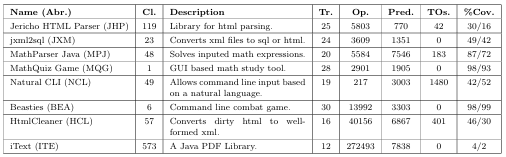
Table 6.1: Program artifacts and constraint descriptions.
We analyzed the artifacts using SSAF and either executed them using the test suite supplied with the artifact or generated and executed our own using the category partition method [29]. This chapter presents the results that our experiments produced for the 174 program traces described in Table 6.1. All experiments were run on a machine with a 2.3 GHz Intel i7 processor running Mac OS X Version 10.8.5 with 8 GB of memory. We used soot version 2.5.0 to instrument our programs. We extended the solvers using Java version 1.6.0 65. ECLiPSe-str was run using the ECLiPSe constraint logic programming environment version 6.1. We used the rst release of Z3-str and JSA version 2.1-1. Finally, we obtained an unnamed release of the STRANGER SML library on December 3, 2013, by contacting the developers1.
6.1 Modeling Cost
We begin by discussing our comparison results on modeling cost, since it does not require an analysis of program traces to measure. Even though Javas string types, i.e., String, StringBuffer, and StringBuilder, have more than 165 methods, we
1At that time STRANGER was not yet open source. It has since been released and is accessible
at https://github.com/vlab-cs-ucsb/Stranger.
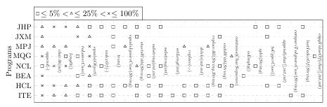
(a) Displays the types and categorizes frequency of methods encountered in DSE for each
source in our test suite.
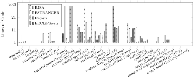
(b) Displays the modeling cost for each method and each extended solver.
Figure 6.1: Uses methods encountered on the x-axis to display modeling cost and characteristics of our test suite.
only present the modeling cost of those string methods that appeared in the execu
equals(Object) indexOf(-) trim() tions of our program traces, while excluding those that have no e ect on symbolic
equalsIgnoreCase(String) startsWith(String) substring(int,int) expressions, such as the toString() method. The total number of unique methods substring(int) set Length(int) used in the traces, other then methods such as toString(), are 33, which we aggre replace(-,-) delete(int,int) replaceAll(String,String) gated to 24 using the wildcard character- to represent overloaded methods, e.g., endsWith(String) contains(CharSequence) append(-) denotes several methods including append(int) and append(boolean). isEmpty() split(String) toUpperCase() append(char[],int,int)
The modeling cost of those methods is the sum of LOC of all aggregated methods.
Figures 6.1a and 6.1b display the encountered string methods on its x-axis. The order of these methods is based on the frequency they appear in all program traces. Thus, append(-) was encountered more often than any other method. The modeling cost in terms of LOC for each string method is shown on the y-axis of the bar graph in Figure 6.1b. If a solver cannot model a method, the corresponding bar is absent. For example, none of the solvers can model charAt(int), and only EJSA and ESTRANGER can model toLowerCase(). The graph shows that, out of 24 aggregated methods, eight of them could not be modeled by any solver2. EJSA was able to model 16 methods, ESTRANGER 16, EZ3-str 12, and ECLiPSe-str 12. The average number of LOC per method modeled is 19.1 for EJSA, 11.9 for ESTRANGER, 5 for EZ3-str, and 5.8 for EECLiPSe-str. The higher number of LOC that is needed for modeling equalsIgnore Case(String), substring (int,int), substring(int), and delete(int,int) methods by EJSA, as well as the lines required to model trim() and equalsIgnoreCase(String) by ESTRANGER, reflect our custom implementation of the substring algorithm in EJSA to increase the solvers precision. Even though EJSA and ESTRANGER required more LOC to model methods, we were able to model more methods due to their available interfaces. So, its no surprise that many analysis tools [37, 33, 14] adapt JSA as the core of their constraint solvers. This implies that users benefit from an extensive interface that can manipulate the solvers underlying representations, but at the same time users might use them incorrectly. ECLiPSe-str does provide an interface that allows us to 2We did not model operations such as charAt(int) because a comparison to a character is required to generate the corresponding constraint. This can be handled by hybrid solvers, which also operate on symbolic integers. For example, in the context of mixed constraints JST can model that method [14].
model more methods as a result of its implementation language, which is a modi ed version of Prolog, but we found it more di cult to use and may not have used it to its full potential. The modeling cost and the importance of precise modeling might vary by program trace, since a trace might use a subset of string methods. Figure 6.1a shows the frequency with which methods appear in PCs of each artifact, which are displayed on the y-axis. The presence of a mark means that the corresponding method was used in the artifacts PCs, while the shape of the mark indicates the prevalence of the method in the artifact. For example, a square implies that the method represents less than 5% of the total number of methods in PCs for that artifact. Using data from the two graphs, we calculated that the average modeling costs for two artifacts could vary signi cantly depending on the solver. Thus, for the MPJ program, the average modeling cost is 17.4 with EJSA and 13.6 with ESTRANGER, while for the HCL program the average modeling cost for EJSA is 20.3 and for ESTRANGER is 10.5, i.e., it takes more modeling cost to extend EJSA for HCL than for MPJ, while the opposite is true for ESTRANGER.
In summary, we nd that on average EZ3-str incurred the lowest modeling cost for our artifacts, i.e., it required the least LOC to extend. EECLiPSe-str came in second followed respectively by ESTRANGER and EJSA. We believe that there are four factors that a ect this result. First, the modeling cost varies by artifact analyzed. Second, Z3-str and ECLiPSe-str directly refer to string constraints while JSA and STRANGER instead focus on automata operations. In fact, a basic knowledge of automata is required to use JSA and STRANGER to their fullest extent. Third, JSA
and STRANGERs interfaces allowed us to more precisely model some methods, but at a high modeling cost. Fourth, Z3-str and ECLiPSe-strs syntaxes require fewer LOC
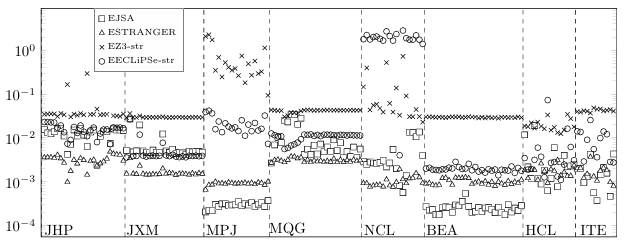
Figure 6.2: Y-axis displays the average time per branching point in seconds.
to express string constraints than Java APIs for string constraints, which are used for both automata-based solvers. Z3-strs syntax is roughly based on the SMT-LIB 2.0 standard [2], and ECLiPSe-strs syntax is based on a functional programming language. These results suggest that a standard format for string constraints, as is proposed in [4], would be bene cial for users of string constraint solvers. Modeling cost would be irrelevant for comparison if all solvers use the same input language.
6.2 Performance
Figure 6.2 displays the average performance of the solvers on PCs gathered at branching points. The y-axis of the graph depicts time in seconds while the x-axis contains all traces grouped by the artifact. The dashed lines indicate the boundaries of program traces and the legend for each constraint solver is presented in the graph. The data shows that the performance varies among solvers for the same artifact, e.g., as in the data for MPJ. In addition, no single constraint solver outperforms all other solvers for all program traces. For each program trace, one of the automata-based
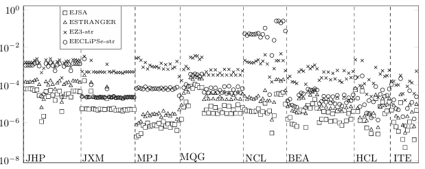
Figure 6.3: Y-axis displays the median time per branching point in seconds.
solvers always exhibits the best performance, with the exception of a couple traces of program HCL. EZ3-str has the worst average performance overall, since for each program trace it either demonstrates the worst performance or it is the close second to worst. EECLiPSE-str has the most variability in its performance. For some artifacts, such as
NCL, it has the worst performance due to timeouts, while for other artifacts, such as JXM, its performance is comparable with the automata-based solvers performance. In addition, the data shows that when a solver has the worst or the best performance for a single program trace, it tends to stay the same in the rest of the program traces for that artifact. Therefore, by sampling PCs of a program trace the user can identify solvers that are more likely to perform well for that artifact. We conjecture that this is due to the string method composition of PCs. Figure 6.3 shows the median performance of the extended solvers on PCs gathered at branching points. The graph uses the same format as Figure 6.2. It shows that the median time for all extended string constraint solvers is at least an order of magnitude lower than the average time for the same program trace. This implies that di cult problems take signi cantly longer to solve than simple problems in all solvers, which increases the average time. In other words, a majority of PCs require much less time to solve than the average time. Also, EJSA always reports the best median time, even though ESTRANGER has a better average time for programs JHP, JXM, and some instances of HCL. This means that ESTRANGER is often less dependent on the complexity of PCs than EJSA. In conclusion, the automata based string constraint solvers often exhibit the best performance, although in some cases EECLiPSe-str outperforms EJSA or ES TRANGER.Inaddition, all solvers su er extreme performance costs on more di cult PCs, although we see that ESTRANGER handles these more di cult PCs well when compared to EJSA.
6.3 Accuracy
Figures 6.5a to 6.5e show the accuracy data derived from the metrics of accuracy introduced in Chapter 3. As in the performance graphs, the x-axis in these gures displays the program traces grouped by artifact. The order of traces in the accuracy graphs are the same as that in the performance graphs. The units in the y-axis of each graph is the percentage of the type of branching points, e.g., disjoint branching points, to the total number of branching points in the trace. In each of these gures, we report the measure of accuracy for each solver. In some cases, we also include the total measure of a particular type of branching point for all of the solvers. Thus, the graph in Figure 6.5a shows the percentage of unsatis able branching points that each solver is able to identify with the solid line representing the total number of unsatis able branching points found by all solvers. The data indicates that EJSA and ESTRANGER identi ed more unsatis able branching than EECLiPSe-str and EZ3-str in every program trace, again with the exception of a couple of traces of HCL where the other two solvers detect the most of these branching points. In addition, neither EJSA nor ESTRANGER reports the most unsatis able branching points in every trace, which mirrors the average performance results in Figure 6.2, Since we want to examine how e ective string solvers are in identifying unsatis able branching points, we want to remove all trivial cases when a PC contains no symbolic values. Earlier we identi ed the branching points whose PCs contain only concrete values as singleton branching points. Thus, in order to identify non-trivial cases of detecting unsatis able branching points, we eliminated all singleton branching points from the unsatis able branching points. The result of this operation is displayed in Figure 6.5b. The data implies that a majority of the unsatis able branching points were detected due to trivial constraints. EZ3-str and EECLiPSe-str were not able to detect as many of these trivial unsatis able branching points because they could not model operations such as toLowerCase and were forced to over-approximate. Hence, solvers might bene t from implementing an additional layer for evaluating concrete constraints, relieving users of the need to implement those checks as part of their analysis tool and increasing accuracy when every symbolic value in a constraint represents exactly one concrete value. At the same time, the graph shows that ESTRANGER was usually able to detect the most unsatis able branching points for non-trivial PCs, particularly for some traces of programs JHP and BEA. However, in some traces of HCL, EJSA detected the most non-trivial branching points, while in other traces of HCL EZ3-str and EECLiPSe-str detect more of these branching points than the other two solvers.
An additional measure of accuracy that we proposed is the number of complete branching points, i.e., accurate disjoint branching points. The graph in Figure 6.5c presents the number of complete branching points, excluding the unsatis able ones, since we analyzed them separately. The data shows that for some program traces, such as those for JHP and MPJ, the results are better for EZ3-str or EECLiPSe-str than for the other solvers. However, for other traces, such as those from programs JXM and ITE, EZ3-str and EECLiPSe-str report worse results than the automata-based solvers. Timeouts affect the cases where EECLiPSe-str and EZ3-str report fewer complete
branching points, while a precise model of methods such as equals(Object) allows them to detect more complete branching points in other cases. This data suggests that a precise model can be bene cial, but a timeout could cause a solver to lose information that would be retained with a less precise model.
Figure 6.5d shows the number of disjoint branching points that are neither unsatis able nor complete. A data point of 0% may imply that all disjoint branching points have either been identi ed as unsatis able/complete or were never observed. By examining the graph in Figure 6.5e, which shows all disjoint branching points, we can dismiss the latter assumption for a majority of the points. By comparing the total number of disjoint branching points to the unidenti ed disjoint branching points, we can state that for some artifacts a solver can detect the majority of disjoint branching points; however, it is not able to detect them with good accuracy, while other solvers can detect fewer disjoint branching points but do it with better accuracy. For example, in JHP EZ3-str and EECLiPSe-str often detect the most new disjoint branching points, but most of EJSA and ESTRANGER s disjoint branching points
are also unsatis able. We see several mixed results in Figure 6.5d. For example, EZ3-str reports the
largest number of unclassi ed disjoint branching points in several traces of NCL and all traces of HCL while the automata-based solver report the most of these branching points for traces of MPJ. These results, along with others, likely depend on the differing PCs within our program traces. When we tracked the number of subset branching points for EJSA and ES TRANGER, we found that all non-disjoint branching points are subset branching points. This might appear suspicious at rst, but it simply means that in these solvers whenever a precise model of a branching point cannot be found at least one branch has the same symbolic value as before the branch. For example, we only model the not equals predicate in these solvers when the argument represents a single concrete value.
We also tracked the top operations for EZ3-str and EECLiPSe-str. However, we observed that both of these solvers always reported the same number of top operations in the program traces. This indicates that they both completely over-approximate the same operations. In addition, the number of top operations varied based on the program trace. For example, we found no top operations for any trace of of MQG or NCL, and we found that at least 20% of the operations in every trace of JXM was a top operation. Overall, no more than 45% of the operations in any trace were top operations. When we combine all of our measurements of accuracy, we see varied results. For example, EJSA and ESTRANGER report the highest percentage of unsatis able branching points for program JHP while EECLiPSe-str reports the highest percentage of complete branching points for the same artifact. Overall, we have identified several cases of accurate branching points within the solvers, along with several cases of over-approximated results. For example, if EJSA reports UNSAT for a PC and EECLiPSe-str reports SAT for the same PC we know that EJSAs result is accurate while EECLiPSe-strs result is not.
6.4 Recommendations
The results presented above suggest that there is no single solver that outperforms other solvers in all of our evaluation criteria. For example, even though EJSA and ESTRANGER supersede the other solvers in performance and detection of unsatis able branching points, they require a higher modeling cost. Therefore, we make several recommendations for users of string constraint solvers. So far, results show that the programs di er in the types of string constraints encountered. For example, program JHP is the only artifact where EECLiPSe-str records the most complete branching points for every trace in Figure 6.5c. Therefore, we suggest the user sample the types of constraints in the program before choosing a string constraint solver.
This sample might be as simple as observing the frequency of each method in a program trace. For example, we see in Figure 6.1a that for MPJ the equals method appears more than 25% of the time but toLowerCase and toUpperCase never occur. We also see that EZ3-str and EECLiPSe-str report the most complete branching points for this program. Thus, we recommend the user use solvers such as EZ3-str and EECLiPSe-str for program traces that have several instances of the equals method but no instance of toLowerCase or toUpperCase. We can observe several examples, in addition to this MPJ example, where the type of constraint appears to a ect results. To start with, we see that in Figure 6.5a that no solvers report any unsatis able branching points for JXM and MQG, and all of the
void o(String s){
if(s.equals(“foo”)){
System.out.println(s.concat(“1”));
return;
}
if(s.equals(“bar”)){
System.out.println(s.concat(“2”));
return;
}
}
Figure 6.4: A code snippet that will not produce unsatis able branching points.
solvers except for EECLiPSe-str report comparable results for other measurements of accuracy. Upon examination of the source code of these programs, we found that whenever an equals predicate was asserted, the corresponding value was immediately processed and consumed, as we see in Figure 6.4. In such programs, an unsatis able branching point will not occur because as soon as a symbolic value is restricted enough to be part of an unsatis able branching point, we do not assert any additional predicates. When this happens, all solvers appear to demonstrate similar accuracy. We propose that the user should choose another metric for determining which solver to use for programs that exhibit the structure in Figure 6.4.
We also see for BEA the accuracy for all of the solvers is almost the same in all measurements. The method distribution in Figure 6.1a shows that, with the exception of equals(Object) and a few instances of toLowerCase(), the program traces contain methods that all solvers handle equivalently. Furthermore, all solvers appear to handle equals and not equals equivalently for BEA. Thus, we recommend that the user use another metric to determine an appropriate solver when he or she suspects that the program contains mostly constraints that will be modeled the same way in all solvers.
We also see that EECLiPSe-str has the fewest unsatis able branching points for NCL. Likewise, it displays the worst performance for this program. We believe this poor accuracy and performance is caused by timeouts that come from more precise models of startsWith() and endsWith(), i.e., even though we attempted to make the solver more accurate, EECLiPSe-str actually lost accuracy due to timeouts. This indicates that in some cases the better model is the one that over-approximates. In addition, the way the constraint is used is just as important as the constraint itself, i.e., there are likely some programs where EECLiPSe-str is the most accurate solver because it has more precise models of these predicates, e.g., it reports the most complete branching points for JHP in Figure 6.5c, which contains instances of startsWith() . Based on this observation, we suggest the user vary the level of precision in his or her extended solvers based on the programs being analyzed. Overall, we see that di erent solvers are successful in di erent situations. For example, the best performance may be achieved by collecting the first result from EJSA or ESTRANGER.
In addition, the best accuracy is likely obtained by using all solvers. For example, EJSA reports the most unsatis able branching points for BEA, ESTRANGER reports the most non-trivial unsatis able branching points for JHP, EECLiPSe-str reports the most complete branching points for MPJ, and EZ3-str reports the most disjoint branching points for HCL. Hence, we recommend the user execute several solvers in parallel in order to get the best performance or accuracy results.
We hope these results are useful in future comparisons of string constraint solvers. They show that string constraint solvers are complex tools involving several factors. In addition, they justify our metrics for string solver comparison presented in Chapter 3 and our approach at measuring those metrics presented in Chapter 5. We proceed to present our overall conclusion in Chapter 7.
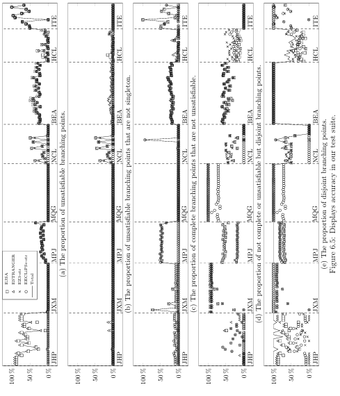
CHAPTER 7
CONCLUSION AND FUTURE WORK
7.1 Comparison of String Constraint Solvers
Traditionally, performance has been the primary means of comparison between string constraint solvers. However, in this thesis we identi ed two new metrics, modeling cost and solver accuracy, that users should consider while identifying an appropriate solver for their needs. We exempli ed comparisons using these metrics on four different extended string constraint solvers: EJSA, ESTRANGER, EZ3-str, and EECLiPSe-str.
In order to produce a comparison of string constraint solvers, we first introduce SE, constraint solvers, string constraint solvers, and DSE in Chapter 1. After that, we present a survey of string constraint solvers, string constraint solver clients, and related work on comparison of these solvers in Chapter 2. We then introduce metrics for comparisons in detail in Chapter 3. Chapter 4 presents SSAF, which we used with the evaluator described in Chapter 5 to perform the comparisons. The results are presented in Chapter 6. Overall, the constraint solvers exhibited a wide variation in the measurements for our metrics; the solvers not only evaluated differently for various metrics, but those variations were dependent on the type of measurement. This suggests that users of constraint solvers for complex types could gain from using several different underlying solvers, depending on the situation.
7.2 Future Work
7.2.1 Comparisons
We would like to perform comparisons on hybrid string constraints. For example, perhaps a solver will report more complete or unsatis able branching points if it can solve predicates based on charAt(int).
We want to investigate further metrics for comparisons of constraint solvers. We would also like to expand research in our current metrics. Speci cally, we plan to continue our work by introducing additional measurements of accuracy for both predicates and operations. Our only current empirical measurement of accuracy on operations records top operations, so we would like to include further measurements on operations.
In particular, we would like to investigate if operations or predicates can remove over-approximation introduced in a previous operation or predicate. For example, substring(int,int) only extracts part of the original value, so perhaps its result captures a portion of the string that is una ected by a not endsWith predicate that was not modeled precisely in EJSA, ESTRANGER, and EZ3-str. In addition, we would like to investigate input values generated using constraint solvers. This would be done by nding solutions for initial symbolic values in a PC. After that, these solutions would be used to follow the path described by the PC. If the values follow the path, then the solutions are correct. We do not use this as a measurement of accuracy because even an inaccurate solver could produce a correct solution for an initial symbolic value. Therefore, we would like to leverage this technique to use it as a measurement of accuracy.
Finally, we would like to determine more information on accuracy at branch ing points. For example, we would like to determine which branch causes over approximation in a non-disjoint branching point. In addition, we would like to investigate extensions of solvers such as Z3-str and ECLiPSe-str that are capable of detecting subsets, i.e., they might allow a constraint that says the language represented by one symbolic value is a subset of the language represented by another. This would allow such solvers to detect subset branching points and additional value branching points.
7.2.2 Constraint Solver Development
We would like to see our experience aid in development of future constraint solvers of complex types and give users a better understanding of string constraint solvers. Primarily, we suggest using several solvers in parallel in order to generate the best results. In addition, we advocate a standardization of the language describing string con straints. This would allow easy parallelization by letting users specify one model for all solvers. Furthermore, it would eliminate modeling cost as a means of comparison. Finally, we suggest a line of future research that focuses on exchanging learned information between solvers. For example, an automata solver might create a regular expression of accepting strings and a bit-vector solver might create a constraint from that regular expression. We believe this approach will improve the accuracy of constraint solvers for all complex data types, not just string types. Passing learned information would also allow more intricate comparisons of accuracy. For example we would be able to determine if the set of values represented by a symbolic value in EJSA is a subset of the set of values represented by a symbolic value in EZ3-str.
7.3 Final Note
We hope that the metrics presented in Chapter 3 will be used in future comparison of constraint solvers. We designed these metrics to be applicable to all constraint solvers, not just string constraint solvers. These metrics are provided to give constraint solver users a comprehensive description of constraint solvers. We provide one such description for several diverse string constraint solvers.
REFERENCES
[1] Sourceforge. http://sourceforge.net/.
[2] Clark Barrett, Aaron Stump, and Cesare Tinelli. The Satis ability Modulo Theories Library (SMT-LIB). www.SMT-LIB.org, 2010.
[3] Morten Biehl, Nils Klarlund, and Theis Rauhe. Algorithms for guided tree automata. In Automata Implementation, pages 625. Springer, 1997.
[4] Nikolaj Bj rner, Vijay Ganesh, Raphael Michel, and Margus Veanes. An smt-lib format for sequences and regular expressions. In Strings, page 24, 2012.
[5] Nikolaj Bj rner, Nikolai Tillmann, and Andrei Voronkov. Path feasibility analysis for string-manipulating programs. In Tools and Algorithms for the Construction and Analysis of Systems, pages 307321. Springer, 2009.
[6] Fabian Buttner and Jordi Cabot. Lightweight string reasoning for ocl. In Modelling Foundations and Applications, pages 244258. Springer, 2012.
[7] Fabian Buttner and Jordi Cabot. Lightweight string reasoning in model nding. Software & Systems Modeling, pages 115, 2013.
[8] Tae-Hyoung Choi, Oukseh Lee, Hyunha Kim, and Kyung-Goo Doh. A practical string analyzer by the widening approach. In Programming Languages and Systems, pages 374388. Springer, 2006.
[9] Aske Simon Christensen, Anders Mller, and Michael I Schwartzbach. Precise analysis of string expressions. Springer, 2003.
[10] L. A. Clarke. A system to generate test data and symbolically execute programs. IEEE Trans. Softw. Eng., 2(3):215222, May 1976.
[11] Leonardo De Moura and Nikolaj Bj rner. Z3: An e cient smt solver. In Tools and Algorithms for the Construction and Analysis of Systems, pages 337340. Springer, 2008.
[12] Michael Emmi, Rupak Majumdar, and Koushik Sen. Dynamic test input generation for database applications. In Proceedings of the 2007 international symposium on Software testing and analysis, pages 151162. ACM, 2007.
[13] Vijay Ganesh and David L Dill. A decision procedure for bit-vectors and arrays. In Computer Aided Veri cation, pages 519531. Springer, 2007.
[14] Indradeep Ghosh, Nastaran Sha ei, Guodong Li, and Wei-Fan Chiang. Jst: an automatic test generation tool for industrial java applications with strings. In Proceedings of the 2013 International Conference on Software Engineering, pages 9921001. IEEE Press, 2013.
[15] Carlos A Gonzalez, F Buttner, Robert Clariso, and Jordi Cabot. Emftocsp: A tool for the lightweight veri cation of emf models. In Software Engineering: Rigorous and Agile Approaches (FormSERA), 2012 Formal Methods in, pages
4450. IEEE, 2012.
[16] William GJ Halfond and Alessandro Orso. Combining static analysis and runtime monitoring to counter sql-injection attacks. In ACM SIGSOFT Software Engineering Notes, volume 30, pages 17. ACM, 2005.
[17] Pieter Hooimeijer and Margus Veanes. An evaluation of automata algorithms for string analysis. In Proceedings of the 12th International Conference on Veri cation, Model Checking, and Abstract Interpretation, VMCAI11, pages 248262, Berlin, Heidelberg, 2011. Springer-Verlag.
[18] Pieter Hooimeijer and Westley Weimer. A decision procedure for subset con straints over regular languages. In ACM Sigplan Notices, volume 44, pages 188198. ACM, 2009.
[19] Pieter Hooimeijer and Westley Weimer. Solving string constraints lazily. In Proceedings of the IEEE/ACM International Conference on Automated Software Engineering, ASE 10, pages 377386, New York, NY, USA, 2010. ACM.
[20] JC Huang. Program instrumentation and software testing. Computer, 11(4):25 32, 1978.
[21] Susmit Jha, Sanjit A Seshia, and Rhishikesh Limaye. On the computational complexity of satis ability solving for string theories. arXiv preprint arXiv:0903.2825, 2009.
[22] Nenad Jovanovic, Christopher Kruegel, and Engin Kirda. Pixy: A static analysis tool for detecting web application vulnerabilities. In Security and Privacy, 2006 IEEE Symposium on, pages 6pp. IEEE, 2006.
[23] Sarfraz Khurshid, Ivan Garca, and Yuk Lai Suen. Repairing structurally complex data. In Model Checking Software, pages 123138. Springer, 2005.
[24] Adam Kiezun, Vijay Ganesh, Philip J Guo, Pieter Hooimeijer, and Michael D Ernst. Hampi: a solver for string constraints. In Proceedings of the eighteenth international symposium on Software testing and analysis, pages 105116. ACM, 2009.
[25] Adam Kiezun, Philip J Guo, Karthick Jayaraman, and Michael D Ernst. Automatic creation of sql injection and cross-site scripting attacks. In Software Engineering, 2009. ICSE 2009. IEEE 31st International Conference on, pages 199209. IEEE, 2009.
[26] James C King. Symbolic execution and program testing. Communications of the ACM, 19(7):385394, 1976.
[27] Guodong Li and Indradeep Ghosh. Pass: String solving with parameterized array and interval automaton. In Hardware and Software: Veri cation and Testing, pages 1531. Springer, 2013.
[28] Yasuhiko Minamide. Static approximation of dynamically generated web pages. In Proceedings of the 14th international conference on World Wide Web, pages 432441. ACM, 2005.
[29] Thomas J. Ostrand and Marc J. Balcer. The category-partition method for spec ifying and generating fuctional tests. Communications of the ACM, 31(6):676 686, 1988.
[30] Corinaing Pasareanu.parti. Symbolic execution and software test http://babel sh.arc.nasa.gov/trac/jpf/raw attachment/wiki/presentations/start/slides-pasareanu.pdf, 2012.
[31] Corina S Pasareanu, Peter C Mehlitz, David H Bushnell, Karen Gundy-Burlet, Michael Lowry, Suzette Person, and Mark Pape. Combining unit-level symbolic execution and system-level concrete execution for testing nasa software. In Pro ceedings of the 2008 international symposium on Software testing and analysis, pages 1526. ACM, 2008.
[32] Corina S Pasareanu and Neha Rungta. Symbolic pathnder: symbolic execution of java bytecode. In Proceedings of the IEEE/ACM international conference on Automated software engineering, pages 179180. ACM, 2010.
[33] Gideon Redelinghuys, Willem Visser, and Jaco Geldenhuys. Symbolic execution of programs with strings. In Proceedings of the South African Institute for Computer Scientists and Information Technologists Conference, pages 139148. ACM, 2012.
[34] Prateek Saxena, Devdatta Akhawe, Steve Hanna, Feng Mao, Stephen McCamant, and Dawn Song. A symbolic execution framework for javascript. In Security and Privacy (SP), 2010 IEEE Symposium on, pages 513528. IEEE, 2010.
[35] Edward J Schwartz, Thanassis Avgerinos, and David Brumley. All you ever wanted to know about dynamic taint analysis and forward symbolic execution (but might have been afraid to ask). In Security and Privacy (SP), 2010 IEEE Symposium on, pages 317331. IEEE, 2010.
[36] Koushik Sen, Darko Marinov, and Gul Agha. Cute: a concolic unit testing engine for c. In Proc. ESEC/FSE, pages 263272, 2005.
[37] Daryl Shannon, Sukant Hajra, Alison Lee, Daiqian Zhan, and Sarfraz Khurshid. Abstracting symbolic execution with string analysis. In Testing: Academic and Industrial Conference Practice and Research Techniques-MUTATION, 2007. TAICPART-MUTATION 2007, pages 1322. IEEE, 2007.
[38] Ofer Strichman. Decision procedures: an algorithmic point of view. Springer, 2010.
[39] A. Stump, T. Weber, and D.R. Cok. SMTEVAL 2013:progress report. http:// sat2013. cs. helsinki.fi/ slides/ SMTEVAL 2013.pdf.
[40] Takaaki Tateishi, Marco Pistoia, and Omer Tripp. Path-and index-sensitive string analysis based on monadic second-order logic. In ISSTA, volume 11, pages 166176, 2011.
[41] Richard Uhler and Nirav Dave. Smten: automatic translation of high-level symbolic computations into smt queries. In Computer Aided Veri cation, pages 678683. Springer, 2013.
[42] Raja Vallee-Rai, Phong Co, Etienne Gagnon, Laurie Hendren, Patrick Lam, and Vijay Sundaresan. Soot: A java bytecode optimization framework. pages 214224, 2010.
[43] Gary Wassermann and Zhendong Su. Sound and precise analysis of web applications for injection vulnerabilities. In ACM Sigplan Notices, volume 42, pages 3241. ACM, 2007.
[44] Gary Wassermann, Dachuan Yu, Ajay Chander, Dinakar Dhurjati, Hiroshi Inamura, and Zhendong Su. Dynamic test input generation for web applications. In Proceedings of the 2008 international symposium on Software testing and analysis, pages 249260. ACM, 2008.
[45] Fang Yu, Muath Alkhalaf, and Tev k Bultan. Stranger: An automata-based string analysis tool for php. In Tools and Algorithms for the Construction and Analysis of Systems, pages 154157. Springer, 2010.
[46] Fang Yu, Muath Alkhalaf, Tev k Bultan, and Oscar H Ibarra. Automata-based symbolic string analysis for vulnerability detection. Formal Methods in System Design, pages 127, 2013.
[47] Fang Yu, Tev k Bultan, Marco Cova, and Oscar H Ibarra. Symbolic string veri cation: An automata-based approach. In Model Checking Software, pages 306324. Springer, 2008.
[48] Fang Yu, Tev k Bultan, and Oscar H Ibarra. Symbolic string veri cation: Combining string analysis and size analysis. In Tools and Algorithms for the Construction and Analysis of Systems, pages 322336. Springer, 2009.
[49] Fang Yu, Tev k Bultan, and Oscar H Ibarra. Relational string veri cation using multi-track automata. International Journal of Foundations of Computer Science, 22(08):19091924, 2011.
[50] Yunhui Zheng, Xiangyu Zhang, and Vijay Ganesh. Z3-str: a z3-based string solver for web application analysis. In Proceedings of the 2013 9th Joint Meeting on Foundations of Software Engineering, pages 114124. ACM, 2013.